Scipy - Region-based Segmentation

Region-based segmentation is a key approach in image processing for dividing an image into meaningful regions based on pixel intensity, color, texture or other features.

In the view of SciPy, region-based segmentation often leverages libraries such as scipy.ndimage and other Python libraries like skimage (scikit-image).

Approaches of Region-Based Segmentation

Region-based segmentation approaches aim to divide an image into meaningful regions based on certain criteria such as intensity, color or texture. Below are the primary approaches and let's see them one by one −

Region Growing

Region Growing is a pixel-based image segmentation method that starts from one or more seed points and grows regions by adding neighboring pixels that satisfy a similarity criterion. This approach is intuitive, simple and widely used in image processing particularly when prior knowledge about the region of interest (ROI) is available.

Key Concepts

Here are the key concepts that we have to learn before proceeding with the Region growing approach −

• Seed points are the foundation of the region-growing algorithm. They are the starting locations from which the segmentation process begins. The choice and placement of seed points are crucial as they determine the quality and extent of the segmented region.
• Growth criteria define the rules for adding new pixels to a region in the region-growing algorithm. These criteria ensure that the region remains consistent and homogeneous based on specific properties like intensity, color or texture. It is important to define growth criteria properly for obtaining meaningful and accurate segmentation results.
• Connectivity is a critical concept in region-based segmentation and image analysis. It defines how pixels (or voxels in 3D) are considered connected to one another based on their spatial arrangement and/or similarity in values. Connectivity determines how regions are formed by grouping pixels into connected components.
• Stopping conditions are essential in region-based segmentation algorithms to define when the segmentation process should halt. These conditions ensure that the algorithm terminates at an appropriate point, preventing over-segmentation or unnecessary computations.

Region Growing Algorithm

The Region Growing algorithm iteratively adds neighboring pixels to an existing region based on a set of criteria such as intensity, color, texture. Below is a detailed step-by-step breakdown of the Region Growing algorithm −

• Initialize: Choose the seed points and define a similarity threshold and Connectivity.
• Region Growing: Add neighboring pixels to the region if they meet the growth criteria and update the region's properties such as mean intensity as pixels are added.
• Repeat: Continue until no new pixels can be added.
• Output: Segmented regions representing different parts of the image.

Example

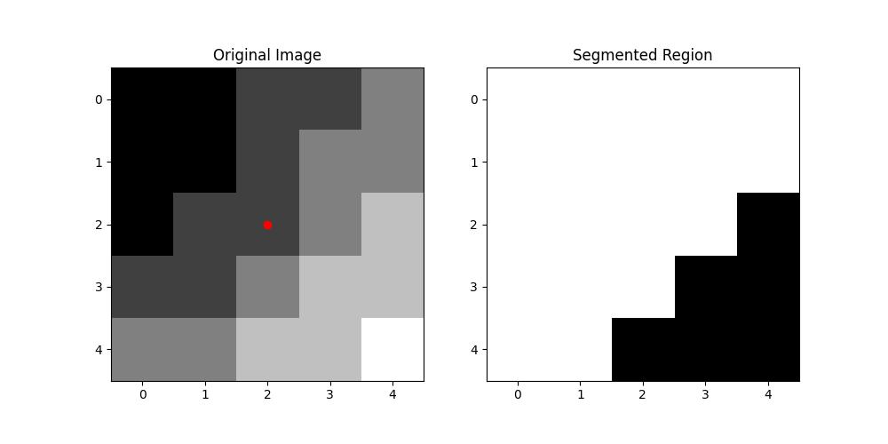
Following is the example which shows how to perform Region Growing approach on an image. In this example we are implementing the region growing for a greyscale image −

 import numpy as np import matplotlib.pyplot as plt def region_growing(image, seed_point, threshold): """ Perform region growing on a grayscale image. Parameters: image (2D numpy array): Input grayscale image. seed_point (tuple): Starting point (row, col) for region growing. threshold (float): Intensity difference threshold for region inclusion. Returns: region (2D numpy array): Binary mask of the segmented region. """ rows, cols = image.shape region = np.zeros_like(image, dtype=bool) visited = np.zeros_like(image, dtype=bool) intensity = image[seed_point] # Initialize the region with the seed point region[seed_point] = True visited[seed_point] = True to_process = [seed_point] while to_process: current_point = to_process.pop(0) r, c = current_point # Check 4-connectivity neighbors for dr, dc in [(-1, 0), (1, 0), (0, -1), (0, 1)]: nr, nc = r + dr, c + dc if 0 <= nr < rows and 0 <= nc < cols and not visited[nr, nc]: visited[nr, nc] = True # Check similarity condition if abs(image[nr, nc] - intensity) <= threshold: region[nr, nc] = True to_process.append((nr, nc)) return region # Example usage if __name__ == "__main__": # Create a synthetic grayscale image image = np.array([[1, 1, 2, 2, 3], [1, 1, 2, 3, 3], [1, 2, 2, 3, 4], [2, 2, 3, 4, 4], [3, 3, 4, 4, 5]], dtype=float) # Define seed point and threshold seed_point = (2, 2) # Starting point in the image threshold = 1.0 # Intensity difference threshold # Apply region growing segmented_region = region_growing(image, seed_point, threshold) # Plot results plt.figure(figsize=(10, 5)) plt.subplot(1, 2, 1) plt.title("Original Image") plt.imshow(image, cmap="gray", interpolation="none") plt.scatter(seed_point[1], seed_point[0], color="red") # Mark seed point plt.subplot(1, 2, 2) plt.title("Segmented Region") plt.imshow(segmented_region, cmap="gray", interpolation="none") plt.show() 

Following is the output of Region Growing approach on a greyscale image −

Region Splitting & Merging

Region Splitting and Merging is a hybrid image segmentation approach that combines top-down and bottom-up techniques. It starts by splitting an image into smaller regions and then merges adjacent regions that satisfy a similarity criterion. This method is particularly useful for hierarchical segmentation and efficiently balances detail and computational effort.

Key Concepts in Region Splitting & Merging

Here are the key concepts that we have to know before proceeding with the Region Splitting and Merging approach −

• Homogeneity criteria define whether a region is uniform based on specific properties such as intensity, color or texture. Proper criteria ensure meaningful and accurate segmentation results.
• Quadtree decomposition is a common splitting method where an image is divided into four quadrants recursively until regions become homogeneous or reach a minimum size.
• Merging criteria determine how adjacent regions are combined. Regions with similar properties are merged to form larger homogeneous areas.
• Stopping conditions are essential to define when splitting or merging should stop by ensuring efficient computation and meaningful segmentation.

Region Splitting & Merging Algorithm

The Region Splitting and Merging algorithm alternates between dividing and combining regions based on defined criteria. Below is a detailed step-by-step breakdown −

• Initialize: Treat the entire image as a single region. Define homogeneity and merging criteria.
• Region Splitting: Recursively divide non-homogeneous regions, typically using quadtree decomposition.
• Region Merging: Combine adjacent homogeneous regions that meet the merging criteria.
• Repeat: Continue splitting and merging until no further changes occur.
• Output: Homogeneous regions representing different parts of the image.

Example

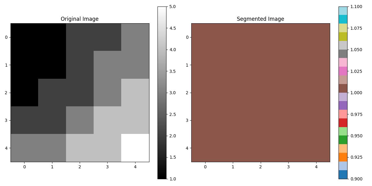
Following is the example which shows how to perform Region Splitting and Merging approach on an image. In this example we are implementing the algorithm using quad-tree decomposition for splitting and simple merging criteria −

 import numpy as np import matplotlib.pyplot as plt from scipy.ndimage import label def is_homogeneous(region, threshold=10): """Check if a region is homogeneous based on intensity variance.""" return np.var(region) < threshold def quadtree_split(image, x, y, size, threshold, segmentation, label_id): """Recursively split a region into quadrants if not homogeneous.""" if size <= 1 or is_homogeneous(image[y:y+size, x:x+size], threshold): segmentation[y:y+size, x:x+size] = label_id return label_id + 1 half = size // 2 label_id = quadtree_split(image, x, y, half, threshold, segmentation, label_id) # Top-left label_id = quadtree_split(image, x + half, y, half, threshold, segmentation, label_id) # Top-right label_id = quadtree_split(image, x, y + half, half, threshold, segmentation, label_id) # Bottom-left label_id = quadtree_split(image, x + half, y + half, half, threshold, segmentation, label_id) # Bottom-right return label_id def region_merge(segmentation, image, threshold): """Merge adjacent regions based on similarity.""" labeled_regions, _ = label(segmentation) region_means = {region: np.mean(image[segmentation == region]) for region in np.unique(segmentation)} for region_a in region_means: for region_b in region_means: if region_a != region_b and abs(region_means[region_a] - region_means[region_b]) < threshold: segmentation[segmentation == region_b] = region_a return segmentation def split_and_merge(image, split_threshold, merge_threshold): """Perform region splitting and merging.""" h, w = image.shape segmentation = np.zeros_like(image, dtype=int) # Perform quadtree splitting label_id = 1 label_id = quadtree_split(image, 0, 0, min(h, w), split_threshold, segmentation, label_id) # Perform merging of regions segmentation = region_merge(segmentation, image, merge_threshold) return segmentation # Example usage if __name__ == "__main__": # Create a synthetic grayscale image image = np.array([[1, 1, 2, 2, 3], [1, 1, 2, 3, 3], [1, 2, 2, 3, 4], [2, 2, 3, 4, 4], [3, 3, 4, 4, 5]], dtype=float) # Define thresholds split_threshold = 1.5 # Variance threshold for splitting merge_threshold = 0.5 # Intensity difference threshold for merging # Apply region splitting and merging segmented_image = split_and_merge(image, split_threshold, merge_threshold) # Plot results plt.figure(figsize=(12, 6)) plt.subplot(1, 2, 1) plt.title("Original Image") plt.imshow(image, cmap="gray", interpolation="none") plt.colorbar() plt.subplot(1, 2, 2) plt.title("Segmented Image") plt.imshow(segmented_image, cmap="tab20", interpolation="none") plt.colorbar() plt.tight_layout() plt.show() 

Following is the output of Region Splitting and Merging approach on a greyscale image −

Watershed Algorithm

The Watershed Algorithm is a segmentation technique in image processing that is inspired by the concept of watershed in topography. It views the image as a topographic surface where pixel intensities represent heights.

This algorithm simulates the process of flooding regions from seed points, with boundaries forming where waters from different seeds meet. The watershed algorithm is commonly used to segment touching or overlapping objects in an image especially in cases where other segmentation methods fail.

Key Concepts of Watershed Algorithm

Here are the key concepts that you need to know before understanding the Watershed Algorithm −

• Topographic Surface represents the image where pixel intensity corresponds to the elevation or height of the surface.
• Gradient Image is derived from the original image and highlights boundaries between regions, essentially simulating the slopes of a topographic map.
• Markers are predefined regions or seed points that are used to guide the flood process. Markers are often placed manually or detected automatically.
• Flooding Process refers to the algorithm's approach of spreading the region from each marker until boundaries are formed.
• Watershed Lines are the boundaries formed where floods from different markers meet, segmenting the image into distinct regions.

Steps in the Watershed Algorithm

The Watershed Algorithm follows a sequence of steps to segment an image. Below is a detailed breakdown −

• Preprocessing: Compute the gradient or edge map of the image to highlight the boundaries between regions.
• Marker Initialization: Mark the initial regions i.e., foreground and background, to define where the flooding process will begin.
• Flooding: Simulate the flooding of regions from each marker. The process continues until the flooded regions meet by forming watershed lines.
• Segmentation: The boundaries formed by the meeting of floods define distinct regions in the image.

Example

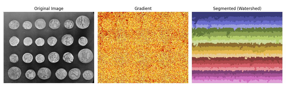
Following is an example that shows how the Watershed Algorithm is applied to an image. In this example we compute the gradient, place markers and then apply the watershed algorithm using scipy −

 import numpy as np import scipy.ndimage as ndi import matplotlib.pyplot as plt from skimage import data, filters, segmentation # Step 1: Load the sample image (e.g., a synthetic image of coins) image = data.coins() # Step 2: Convert the image to grayscale (if it is not already) # Skimage provides the image in grayscale, so we can skip this step. # Step 3: Compute the gradient of the image using a Sobel filter # The gradient will highlight the boundaries (edges) between regions gradient = np.sqrt(ndi.sobel(image, axis=0)**2 + ndi.sobel(image, axis=1)**2) # Step 4: Apply a threshold to create markers for the watershed algorithm # Here we use a simple method: identifying regions with low gradient as markers threshold = filters.threshold_otsu(gradient) markers = gradient < threshold # Step 5: Label markers (background and foreground) # Background will be labeled as 0 and the foreground as 1 markers = ndi.label(markers)[0] # Step 6: Perform the watershed transformation using the gradient image # Watershed labels the regions based on the gradient and the markers labels = segmentation.watershed(gradient, markers) # Step 7: Visualize the results # Plot original image, gradient, and segmented (labeled) result fig, ax = plt.subplots(1, 3, figsize=(12, 4)) ax[0].imshow(image, cmap='gray') ax[0].set_title('Original Image') ax[1].imshow(gradient, cmap='hot') ax[1].set_title('Gradient') ax[2].imshow(labels, cmap='tab20b') ax[2].set_title('Segmented (Watershed)') for a in ax: a.axis('off') plt.tight_layout() plt.show() 

Following is the output of Watershed Algorithm applied to an image −