- ML - Home
- ML - Introduction
- ML - Getting Started
- ML - Basic Concepts
- ML - Ecosystem
- ML - Python Libraries
- ML - Applications
- ML - Life Cycle
- ML - Required Skills
- ML - Implementation
- ML - Challenges & Common Issues
- ML - Limitations
- ML - Reallife Examples
- ML - Data Structure
- ML - Mathematics
- ML - Artificial Intelligence
- ML - Neural Networks
- ML - Deep Learning
- ML - Getting Datasets
- ML - Categorical Data
- ML - Data Loading
- ML - Data Understanding
- ML - Data Preparation
- ML - Models
- ML - Supervised Learning
- ML - Unsupervised Learning
- ML - Semi-supervised Learning
- ML - Reinforcement Learning
- ML - Supervised vs. Unsupervised
- Machine Learning Data Visualization
- ML - Data Visualization
- ML - Histograms
- ML - Density Plots
- ML - Box and Whisker Plots
- ML - Correlation Matrix Plots
- ML - Scatter Matrix Plots
- Statistics for Machine Learning
- ML - Statistics
- ML - Mean, Median, Mode
- ML - Standard Deviation
- ML - Percentiles
- ML - Data Distribution
- ML - Skewness and Kurtosis
- ML - Bias and Variance
- ML - Hypothesis
- Regression Analysis In ML
- ML - Regression Analysis
- ML - Linear Regression
- ML - Simple Linear Regression
- ML - Multiple Linear Regression
- ML - Polynomial Regression
- Classification Algorithms In ML
- ML - Classification Algorithms
- ML - Logistic Regression
- ML - K-Nearest Neighbors (KNN)
- ML - Naïve Bayes Algorithm
- ML - Decision Tree Algorithm
- ML - Support Vector Machine
- ML - Random Forest
- ML - Confusion Matrix
- ML - Stochastic Gradient Descent
- Clustering Algorithms In ML
- ML - Clustering Algorithms
- ML - Centroid-Based Clustering
- ML - K-Means Clustering
- ML - K-Medoids Clustering
- ML - Mean-Shift Clustering
- ML - Hierarchical Clustering
- ML - Density-Based Clustering
- ML - DBSCAN Clustering
- ML - OPTICS Clustering
- ML - HDBSCAN Clustering
- ML - BIRCH Clustering
- ML - Affinity Propagation
- ML - Distribution-Based Clustering
- ML - Agglomerative Clustering
- Dimensionality Reduction In ML
- ML - Dimensionality Reduction
- ML - Feature Selection
- ML - Feature Extraction
- ML - Backward Elimination
- ML - Forward Feature Construction
- ML - High Correlation Filter
- ML - Low Variance Filter
- ML - Missing Values Ratio
- ML - Principal Component Analysis
- Reinforcement Learning
- ML - Reinforcement Learning Algorithms
- ML - Exploitation & Exploration
- ML - Q-Learning
- ML - REINFORCE Algorithm
- ML - SARSA Reinforcement Learning
- ML - Actor-critic Method
- ML - Monte Carlo Methods
- ML - Temporal Difference
- Deep Reinforcement Learning
- ML - Deep Reinforcement Learning
- ML - Deep Reinforcement Learning Algorithms
- ML - Deep Q-Networks
- ML - Deep Deterministic Policy Gradient
- ML - Trust Region Methods
- Quantum Machine Learning
- ML - Quantum Machine Learning
- ML - Quantum Machine Learning with Python
- Machine Learning Miscellaneous
- ML - Performance Metrics
- ML - Automatic Workflows
- ML - Boost Model Performance
- ML - Gradient Boosting
- ML - Bootstrap Aggregation (Bagging)
- ML - Cross Validation
- ML - AUC-ROC Curve
- ML - Grid Search
- ML - Data Scaling
- ML - Train and Test
- ML - Association Rules
- ML - Apriori Algorithm
- ML - Gaussian Discriminant Analysis
- ML - Cost Function
- ML - Bayes Theorem
- ML - Precision and Recall
- ML - Adversarial
- ML - Stacking
- ML - Epoch
- ML - Perceptron
- ML - Regularization
- ML - Overfitting
- ML - P-value
- ML - Entropy
- ML - MLOps
- ML - Data Leakage
- ML - Monetizing Machine Learning
- ML - Types of Data
- Machine Learning - Resources
- ML - Quick Guide
- ML - Cheatsheet
- ML - Interview Questions
- ML - Useful Resources
- ML - Discussion
Machine Learning - Automatic Workflows
Introduction
In order to execute and produce results successfully, a machine learning model must automate some standard workflows. The process of automate these standard workflows can be done with the help of Scikit-learn Pipelines. From a data scientists perspective, pipeline is a generalized, but very important concept. It basically allows data flow from its raw format to some useful information. The working of pipelines can be understood with the help of following diagram −
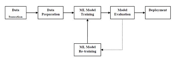
The blocks of ML pipelines are as follows −
Data ingestion − As the name suggests, it is the process of importing the data for use in ML project. The data can be extracted in real time or batches from single or multiple systems. It is one of the most challenging steps because the quality of data can affect the whole ML model.
Data Preparation − After importing the data, we need to prepare data to be used for our ML model. Data preprocessing is one of the most important technique of data preparation.
ML Model Training − Next step is to train our ML model. We have various ML algorithms like supervised, unsupervised, reinforcement to extract the features from data, and make predictions.
Model Evaluation − Next, we need to evaluate the ML model. In case of AutoML pipeline, ML model can be evaluated with the help of various statistical methods and business rules.
ML Model retraining − In case of AutoML pipeline, it is not necessary that the first model is best one. The first model is considered as a baseline model and we can train it repeatably to increase models accuracy.
Deployment − At last, we need to deploy the model. This step involves applying and migrating the model to business operations for their use.
Challenges Accompanying ML Pipelines
In order to create ML pipelines, data scientists face many challenges. These challenges fall into the following three categories −
Quality of Data
The success of any ML model depends heavily on the quality of data. If the data we are providing to ML model is not accurate, reliable and robust, then we are going to end with wrong or misleading output.
Data Reliability
Another challenge associated with ML pipelines is the reliability of data we are providing to the ML model. As we know, there can be various sources from which data scientist can acquire data but to get the best results, it must be assured that the data sources are reliable and trusted.
Data Accessibility
To get the best results out of ML pipelines, the data itself must be accessible which requires consolidation, cleansing and curation of data. As a result of data accessibility property, metadata will be updated with new tags.
Modelling ML Pipeline and Data Preparation
Data leakage, happening from training dataset to testing dataset, is an important issue for data scientist to deal with while preparing data for ML model. Generally, at the time of data preparation, data scientist uses techniques like standardization or normalization on entire dataset before learning. But these techniques cannot help us from the leakage of data because the training dataset would have been influenced by the scale of the data in the testing dataset.
By using ML pipelines, we can prevent this data leakage because pipelines ensure that data preparation like standardization is constrained to each fold of our cross-validation procedure.
Example
The following is an example in Python that demonstrate data preparation and model evaluation workflow. For this purpose, we are using Pima Indian Diabetes dataset from Sklearn. First, we will be creating pipeline that standardized the data. Then a Linear Discriminative analysis model will be created and at last the pipeline will be evaluated using 10-fold cross validation.
First, import the required packages as follows −
from pandas import read_csv from sklearn.model_selection import KFold from sklearn.model_selection import cross_val_score from sklearn.preprocessing import StandardScaler from sklearn.pipeline import Pipeline from sklearn.discriminant_analysis import LinearDiscriminantAnalysis
Now, we need to load the Pima diabetes dataset as did in previous examples −
path = r"C:\pima-indians-diabetes.csv" headernames = ['preg', 'plas', 'pres', 'skin', 'test', 'mass', 'pedi', 'age', 'class'] data = read_csv(path, names=headernames) array = data.values
Next, we will create a pipeline with the help of the following code −
estimators = [] estimators.append(('standardize', StandardScaler())) estimators.append(('lda', LinearDiscriminantAnalysis())) model = Pipeline(estimators) At last, we are going to evaluate this pipeline and output its accuracy as follows −
kfold = KFold(n_splits=20, random_state=7) results = cross_val_score(model, X, Y, cv=kfold) print(results.mean())
Output
0.7790148448043184
The above output is the summary of accuracy of the setup on the dataset.
Modelling ML Pipeline and Feature Extraction
Data leakage can also happen at feature extraction step of ML model. That is why feature extraction procedures should also be restricted to stop data leakage in our training dataset. As in the case of data preparation, by using ML pipelines, we can prevent this data leakage also. FeatureUnion, a tool provided by ML pipelines can be used for this purpose.
Example
The following is an example in Python that demonstrates feature extraction and model evaluation workflow. For this purpose, we are using Pima Indian Diabetes dataset from Sklearn.
First, 3 features will be extracted with PCA (Principal Component Analysis). Then, 6 features will be extracted with Statistical Analysis. After feature extraction, result of multiple feature selection and extraction procedures will be combined by using
FeatureUnion tool. At last, a Logistic Regression model will be created, and the pipeline will be evaluated using 10-fold cross validation.
First, import the required packages as follows −
from pandas import read_csv from sklearn.model_selection import KFold from sklearn.model_selection import cross_val_score from sklearn.pipeline import Pipeline from sklearn.pipeline import FeatureUnion from sklearn.linear_model import LogisticRegression from sklearn.decomposition import PCA from sklearn.feature_selection import SelectKBest
Now, we need to load the Pima diabetes dataset as did in previous examples −
path = r"C:\pima-indians-diabetes.csv" headernames = ['preg', 'plas', 'pres', 'skin', 'test', 'mass', 'pedi', 'age', 'class'] data = read_csv(path, names=headernames) array = data.values
Next, feature union will be created as follows −
features = [] features.append(('pca', PCA(n_components=3))) features.append(('select_best', SelectKBest(k=6))) feature_union = FeatureUnion(features) Next, pipeline will be creating with the help of following script lines −
estimators = [] estimators.append(('feature_union', feature_union)) estimators.append(('logistic', LogisticRegression())) model = Pipeline(estimators) At last, we are going to evaluate this pipeline and output its accuracy as follows −
kfold = KFold(n_splits=20, random_state=7) results = cross_val_score(model, X, Y, cv=kfold) print(results.mean())
Output
0.7789811066126855
The above output is the summary of accuracy of the setup on the dataset.