Performance Metrics in Machine Learning

Performance metrics in machine learning are used to evaluate the performance of a machine learning model. These metrics provide quantitative measures to assess how well a model is performing and to compare the performance of different models. Performance metrics are important because they help us understand how well our model is performing and whether it is meeting our requirements. In this way, we can make informed decisions about whether to use a particular model or not.

We must carefully choose the metrics for evaluating ML performance because −

How the performance of ML algorithms is measured and compared will be dependent entirely on the metric you choose.
How you weight the importance of various characteristics in the result will be influenced completely by the metric you choose.

There are various metrics which we can use to evaluate the performance of ML algorithms, classification as well as regression algorithms. Let's discuss these metrics for Classification and Regression problems separately.

Performance Metrics for Classification Problems

We have discussed classification and its algorithms in the previous chapters. Here, we are going to discuss various performance metrics that can be used to evaluate predictions for classification problems.

Confusion Matrix

The consfusion matrix is the easiest way to measure the performance of a classification problem where the output can be of two or more type of classes. A confusion matrix is nothing but a table with two dimensions viz. "Actual" and "Predicted" and furthermore, both the dimensions have "True Positives (TP)", "True Negatives (TN)", "False Positives (FP)", "False Negatives (FN)" as shown below −

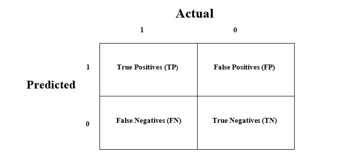
Explanation of the terms associated with confusion matrix are as follows −

True Positives (TP) − It is the case when both actual class & predicted class of data point is 1.
True Negatives (TN) − It is the case when both actual class & predicted class of data point is 0.
False Positives (FP) − It is the case when actual class of data point is 0 & predicted class of data point is 1.
False Negatives (FN) − It is the case when actual class of data point is 1 & predicted class of data point is 0.

We can use confusion_matrix function of sklearn.metrics to compute Confusion Matrix of our classification model.

Classification Accuracy

Accuracy is most common performance metric for classification algorithms. It may be defined as the number of correct predictions made as a ratio of all predictions made. We can easily calculate it by confusion matrix with the help of following formula −

$$Accuracy =\frac{TP+TN}{+++}$$

We can use accuracy_score function of sklearn.metrics to compute accuracy of our classification model.

Classification Report

This report consists of the scores of Precisions, Recall, F1 and Support. They are explained as follows −

Precision

Precision measures the proportion of true positive instances out of all predicted positive instances. It is calculated as the number of true positive instances divided by the sum of true positive and false positive instances.

We can easily calculate it by confusion matrix with the help of following formula −

$$Precision=\frac{TP}{TP+FP}$$

Precision, used in document retrievals, may be defined as the number of correct documents returned by our ML model.

Recall or Sensitivity

Recall measures the proportion of true positive instances out of all actual positive instances. It is calculated as the number of true positive instances divided by the sum of true positive and false negative instances.

We can easily calculate it by confusion matrix with the help of following formula −

$$Recall =\frac{TP}{TP+FN}$$

Specificity

Specificity, in contrast to recall, may be defined as the number of negatives returned by our ML model. We can easily calculate it by confusion matrix with the help of following formula −

$$Specificity =\frac{TN}{TN+FP}$$

Support

Support may be defined as the number of samples of the true response that lies in each class of target values.

F1 Score

F1 score is the harmonic mean of precision and recall. It is a balanced measure that takes into account both precision and recall. Mathematically, F1 score is the weighted average of the precision and recall. The best value of F1 would be 1 and worst would be 0. We can calculate F1 score with the help of following formula −

$$ = ( ) / ( + )$$

F1 score is having equal relative contribution of precision and recall.

We can use classification_report function of sklearn.metrics to get the classification report of our classification model.

ROC AUC Score

The ROC (Receiver Operating Characteristic) Area Under the Curve(AUC) score is a measure of the ability of a classifier to distinguish between positive and negative instances. It is calculated by plotting the true positive rate against the false positive rate at different classification thresholds and calculating the area under the curve.

As name suggests, ROC is a probability curve and AUC measure the separability. In simple words, ROC-AUC score will tell us about the capability of model in distinguishing the classes. Higher the score, better the model.

We can use roc_auc_score function of sklearn.metrics to compute AUC-ROC.

LOGLOSS (Logarithmic Loss)

It is also called Logistic regression loss or cross-entropy loss. It basically defined on probability estimates and measures the performance of a classification model where the input is a probability value between 0 and 1. It can be understood more clearly by differentiating it with accuracy. As we know that accuracy is the count of predictions (predicted value = actual value) in our model whereas Log Loss is the amount of uncertainty of our prediction based on how much it varies from the actual label. With the help of Log Loss value, we can have more accurate view of the performance of our model. We can use log_loss function of sklearn.metrics to compute Log Loss.

Example

The following is a simple recipe in Python which will give us an insight about how we can use the above explained performance metrics on binary classification model −

 from sklearn.metrics import confusion_matrix from sklearn.metrics import accuracy_score from sklearn.metrics import classification_report from sklearn.metrics import roc_auc_score from sklearn.metrics import log_loss X_actual = [1, 1, 0, 1, 0, 0, 1, 0, 0, 0] Y_predic = [1, 0, 1, 1, 1, 0, 1, 1, 0, 0] results = confusion_matrix(X_actual, Y_predic) print ('Confusion Matrix :') print(results) print ('Accuracy Score is',accuracy_score(X_actual, Y_predic)) print ('Classification Report : ') print (classification_report(X_actual, Y_predic)) print('AUC-ROC:',roc_auc_score(X_actual, Y_predic)) print('LOGLOSS Value is',log_loss(X_actual, Y_predic))

Output

 Confusion Matrix : [ [3 3] [1 3] ] Accuracy Score is 0.6 Classification Report : precision recall f1-score support 0 0.75 0.50 0.60 6 1 0.50 0.75 0.60 4 micro avg 0.60 0.60 0.60 10 macro avg 0.62 0.62 0.60 10 weighted avg 0.65 0.60 0.60 10 AUC-ROC: 0.625 LOGLOSS Value is 13.815750437193334

Performance Metrics for Regression Problems

We have discussed regression and its algorithms in previous chapters. Here, we are going to discuss various performance metrics that can be used to evaluate predictions for regression problems.

Mean Absolute Error (MAE)

It is the simplest error metric used in regression problems. It is basically the sum of average of the absolute difference between the predicted and actual values. In simple words, with MAE, we can get an idea of how wrong the predictions were. MAE does not indicate the direction of the model i.e. no indication about underperformance or overperformance of the model. The following is the formula to calculate MAE −

$$MAE = \frac{1}{n}\sum|Y -\hat{Y}|$$

Here, =Actual Output Values

And $\hat{Y}$= Predicted Output Values.

We can use mean_absolute_error function of sklearn.metrics to compute MAE.

Mean Square Error (MSE)

MSE is like the MAE, but the only difference is that the it squares the difference of actual and predicted output values before summing them all instead of using the absolute value. The difference can be noticed in the following equation −

$$MSE = \frac{1}{n}\sum(Y -\hat{Y})$$

Here, =Actual Output Values

And $\hat{Y}$ = Predicted Output Values.

We can use mean_squared_error function of sklearn.metrics to compute MSE.

R Squared (R²) Score

R Squared metric is generally used for explanatory purpose and provides an indication of the goodness or fit of a set of predicted output values to the actual output values. The following formula will help us understanding it −

$$R^{2} = 1 -\frac{\frac{1}{n}\sum_{i{=1}}^n(Y_{i}-\hat{Y_{i}})^2}{\frac{1}{n}\sum_{i{=1}}^n(Y_{i}-\bar{Y_i)^2}}$$

In the above equation, numerator is MSE and the denominator is the variance in values.

We can use r2_score function of sklearn.metrics to compute R squared value.

Example

The following is a simple recipe in Python which will give us an insight about how we can use the above explained performance metrics on regression model −

 from sklearn.metrics import r2_score from sklearn.metrics import mean_absolute_error from sklearn.metrics import mean_squared_error X_actual = [5, -1, 2, 10] Y_predic = [3.5, -0.9, 2, 9.9] print ('R Squared =',r2_score(X_actual, Y_predic)) print ('MAE =',mean_absolute_error(X_actual, Y_predic)) print ('MSE =',mean_squared_error(X_actual, Y_predic))

Output

 R Squared = 0.9656060606060606 MAE = 0.42499999999999993 MSE = 0.5674999999999999

Print Page

Performance Metrics in Machine Learning