- ML - Home
- ML - Introduction
- ML - Getting Started
- ML - Basic Concepts
- ML - Ecosystem
- ML - Python Libraries
- ML - Applications
- ML - Life Cycle
- ML - Required Skills
- ML - Implementation
- ML - Challenges & Common Issues
- ML - Limitations
- ML - Reallife Examples
- ML - Data Structure
- ML - Mathematics
- ML - Artificial Intelligence
- ML - Neural Networks
- ML - Deep Learning
- ML - Getting Datasets
- ML - Categorical Data
- ML - Data Loading
- ML - Data Understanding
- ML - Data Preparation
- ML - Models
- ML - Supervised Learning
- ML - Unsupervised Learning
- ML - Semi-supervised Learning
- ML - Reinforcement Learning
- ML - Supervised vs. Unsupervised
- Machine Learning Data Visualization
- ML - Data Visualization
- ML - Histograms
- ML - Density Plots
- ML - Box and Whisker Plots
- ML - Correlation Matrix Plots
- ML - Scatter Matrix Plots
- Statistics for Machine Learning
- ML - Statistics
- ML - Mean, Median, Mode
- ML - Standard Deviation
- ML - Percentiles
- ML - Data Distribution
- ML - Skewness and Kurtosis
- ML - Bias and Variance
- ML - Hypothesis
- Regression Analysis In ML
- ML - Regression Analysis
- ML - Linear Regression
- ML - Simple Linear Regression
- ML - Multiple Linear Regression
- ML - Polynomial Regression
- Classification Algorithms In ML
- ML - Classification Algorithms
- ML - Logistic Regression
- ML - K-Nearest Neighbors (KNN)
- ML - Naïve Bayes Algorithm
- ML - Decision Tree Algorithm
- ML - Support Vector Machine
- ML - Random Forest
- ML - Confusion Matrix
- ML - Stochastic Gradient Descent
- Clustering Algorithms In ML
- ML - Clustering Algorithms
- ML - Centroid-Based Clustering
- ML - K-Means Clustering
- ML - K-Medoids Clustering
- ML - Mean-Shift Clustering
- ML - Hierarchical Clustering
- ML - Density-Based Clustering
- ML - DBSCAN Clustering
- ML - OPTICS Clustering
- ML - HDBSCAN Clustering
- ML - BIRCH Clustering
- ML - Affinity Propagation
- ML - Distribution-Based Clustering
- ML - Agglomerative Clustering
- Dimensionality Reduction In ML
- ML - Dimensionality Reduction
- ML - Feature Selection
- ML - Feature Extraction
- ML - Backward Elimination
- ML - Forward Feature Construction
- ML - High Correlation Filter
- ML - Low Variance Filter
- ML - Missing Values Ratio
- ML - Principal Component Analysis
- Reinforcement Learning
- ML - Reinforcement Learning Algorithms
- ML - Exploitation & Exploration
- ML - Q-Learning
- ML - REINFORCE Algorithm
- ML - SARSA Reinforcement Learning
- ML - Actor-critic Method
- ML - Monte Carlo Methods
- ML - Temporal Difference
- Deep Reinforcement Learning
- ML - Deep Reinforcement Learning
- ML - Deep Reinforcement Learning Algorithms
- ML - Deep Q-Networks
- ML - Deep Deterministic Policy Gradient
- ML - Trust Region Methods
- Quantum Machine Learning
- ML - Quantum Machine Learning
- ML - Quantum Machine Learning with Python
- Machine Learning Miscellaneous
- ML - Performance Metrics
- ML - Automatic Workflows
- ML - Boost Model Performance
- ML - Gradient Boosting
- ML - Bootstrap Aggregation (Bagging)
- ML - Cross Validation
- ML - AUC-ROC Curve
- ML - Grid Search
- ML - Data Scaling
- ML - Train and Test
- ML - Association Rules
- ML - Apriori Algorithm
- ML - Gaussian Discriminant Analysis
- ML - Cost Function
- ML - Bayes Theorem
- ML - Precision and Recall
- ML - Adversarial
- ML - Stacking
- ML - Epoch
- ML - Perceptron
- ML - Regularization
- ML - Overfitting
- ML - P-value
- ML - Entropy
- ML - MLOps
- ML - Data Leakage
- ML - Monetizing Machine Learning
- ML - Types of Data
- Machine Learning - Resources
- ML - Quick Guide
- ML - Cheatsheet
- ML - Interview Questions
- ML - Useful Resources
- ML - Discussion
Random Forest Algorithm in Machine Learning
Random Forest is a machine learning algorithm that uses an ensemble of decision trees to make predictions. The algorithm was first introduced by Leo Breiman in 2001. The key idea behind the algorithm is to create a large number of decision trees, each of which is trained on a different subset of the data. The predictions of these individual trees are then combined to produce a final prediction.
Working of Random Forest Algorithm
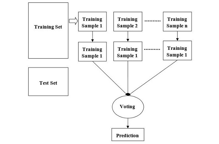
We can understand the working of Random Forest algorithm with the help of following steps −
Step 1 − First, start with the selection of random samples from a given dataset.
Step 2 − Next, this algorithm will construct a decision tree for every sample. Then it will get the prediction result from every decision tree.
Step 3 − In this step, voting will be performed for every predicted result.
Step 4 − At last, select the most voted prediction result as the final prediction result.
The following diagram illustrates how the Random Forest Algorithm works −
Random Forest is a flexible algorithm that can be used for both classification and regression tasks. In classification tasks, the algorithm uses the mode of the predictions of the individual trees to make the final prediction. In regression tasks, the algorithm uses the mean of the predictions of the individual trees.
Advantages of Random Forest Algorithm
Random Forest algorithm has several advantages over other machine learning algorithms. Some of the key advantages are −
Robustness to Overfitting − Random Forest algorithm is known for its robustness to overfitting. This is because the algorithm uses an ensemble of decision trees, which helps to reduce the impact of outliers and noise in the data.
High Accuracy − Random Forest algorithm is known for its high accuracy. This is because the algorithm combines the predictions of multiple decision trees, which helps to reduce the impact of individual decision trees that may be biased or inaccurate.
Handles Missing Data − Random Forest algorithm can handle missing data without the need for imputation. This is because the algorithm only considers the features that are available for each data point and does not require all features to be present for all data points.
Non-Linear Relationships − Random Forest algorithm can handle non-linear relationships between the features and the target variable. This is because the algorithm uses decision trees, which can model non-linear relationships.
Feature Importance − Random Forest algorithm can provide information about the importance of each feature in the model. This information can be used to identify the most important features in the data and can be used for feature selection and feature engineering.
Implementation of Random Forest Algorithm in Python
Let's take a look at the implementation of Random Forest Algorithm in Python. We will be using the scikit-learn library to implement the algorithm. The scikit-learn library is a popular machine learning library that provides a wide range of algorithms and tools for machine learning.
Step 1 − Importing the Libraries
We will begin by importing the necessary libraries. We will be using the pandas library for data manipulation, and the scikit-learn library for implementing the Random Forest algorithm.
import pandas as pd from sklearn.ensemble import RandomForestClassifier
Step 2 − Loading the Data
Next, we will load the data into a pandas dataframe. For this tutorial, we will be using the famous Iris dataset, which is a classic dataset for classification tasks.
# Loading the iris dataset iris = pd.read_csv('https://archive.ics.uci.edu/ml/machine-learningdatabases/iris/iris.data', header=None) iris.columns = ['sepal_length', 'sepal_width', 'petal_length','petal_width', 'species'] Step 3 − Data Preprocessing
Before we can use the data to train our model, we need to preprocess it. This involves separating the features and the target variable and splitting the data into training and testing sets.
# Separating the features and target variable X = iris.iloc[:, :-1] y = iris.iloc[:, -1] # Splitting the data into training and testing sets from sklearn.model_selection import train_test_split X_train, X_test, y_train, y_test = train_test_split(X, y, test_size=0.35, random_state=42)
Step 4 − Training the Model
Next, we will train our Random Forest classifier on the training data.
# Creating the Random Forest classifier object rfc = RandomForestClassifier(n_estimators=100) # Training the model on the training data rfc.fit(X_train, y_train)
Step 5 − Making Predictions
Once we have trained our model, we can use it to make predictions on the test data.
# Making predictions on the test data y_pred = rfc.predict(X_test)
Step 6 − Evaluating the Model
Finally, we will evaluate the performance of our model using various metrics such as accuracy, precision, recall, and F1-score.
# Importing the metrics library from sklearn.metrics import accuracy_score, precision_score, recall_score, f1_score # Calculating the accuracy, precision, recall, and F1-score accuracy = accuracy_score(y_test, y_pred) precision = precision_score(y_test, y_pred, average='weighted') recall = recall_score(y_test, y_pred, average='weighted') f1 = f1_score(y_test, y_pred, average='weighted') print("Accuracy:", accuracy) print("Precision:", precision) print("Recall:", recall) print("F1-score:", f1) Complete Implementation Example
Below is the complete implementation example of Random Forest Algorithm in python using the iris dataset −
import pandas as pd from sklearn.ensemble import RandomForestClassifier # Loading the iris dataset iris = pd.read_csv('https://archive.ics.uci.edu/ml/machine-learningdatabases/iris/iris.data', header=None) iris.columns = ['sepal_length', 'sepal_width', 'petal_length', 'petal_width', 'species'] # Separating the features and target variable X = iris.iloc[:, :-1] y = iris.iloc[:, -1] # Splitting the data into training and testing sets from sklearn.model_selection import train_test_split X_train, X_test, y_train, y_test = train_test_split(X, y, test_size=0.35, random_state=42) # Creating the Random Forest classifier object rfc = RandomForestClassifier(n_estimators=100) # Training the model on the training data rfc.fit(X_train, y_train) # Making predictions on the test data y_pred = rfc.predict(X_test) # Importing the metrics library from sklearn.metrics import accuracy_score, precision_score, recall_score, f1_score # Calculating the accuracy, precision, recall, and F1-score accuracy = accuracy_score(y_test, y_pred) precision = precision_score(y_test, y_pred, average='weighted') recall = recall_score(y_test, y_pred, average='weighted') f1 = f1_score(y_test, y_pred, average='weighted') print("Accuracy:", accuracy) print("Precision:", precision) print("Recall:", recall) print("F1-score:", f1) Output
This will give us the performance metrics of our Random Forest classifier as follows −
Accuracy: 0.9811320754716981 Precision: 0.9821802935010483 Recall: 0.9811320754716981 F1-score: 0.9811157396063056
Pros and Cons of Random Forest
Pros
The following are the advantages of Random Forest algorithm −
It overcomes the problem of overfitting by averaging or combining the results of different decision trees.
Random forests work well for a large range of data items than a single decision tree does.
Random forest has less variance then single decision tree.
Random forests are very flexible and possess very high accuracy.
Scaling of data does not require in random forest algorithm. It maintains good accuracy even after providing data without scaling.
Scaling of data does not require in random forest algorithm. It maintains good accuracy even after providing data without scaling.
Cons
The following are the disadvantages of Random Forest algorithm −
Complexity is the main disadvantage of Random forest algorithms.
Construction of Random forests are much harder and time-consuming than decision trees.
More computational resources are required to implement Random Forest algorithm.
It is less intuitive in case when we have a large collection of decision trees .
The prediction process using random forests is very time-consuming in comparison with other algorithms.