- ML - Home
- ML - Introduction
- ML - Getting Started
- ML - Basic Concepts
- ML - Ecosystem
- ML - Python Libraries
- ML - Applications
- ML - Life Cycle
- ML - Required Skills
- ML - Implementation
- ML - Challenges & Common Issues
- ML - Limitations
- ML - Reallife Examples
- ML - Data Structure
- ML - Mathematics
- ML - Artificial Intelligence
- ML - Neural Networks
- ML - Deep Learning
- ML - Getting Datasets
- ML - Categorical Data
- ML - Data Loading
- ML - Data Understanding
- ML - Data Preparation
- ML - Models
- ML - Supervised Learning
- ML - Unsupervised Learning
- ML - Semi-supervised Learning
- ML - Reinforcement Learning
- ML - Supervised vs. Unsupervised
- Machine Learning Data Visualization
- ML - Data Visualization
- ML - Histograms
- ML - Density Plots
- ML - Box and Whisker Plots
- ML - Correlation Matrix Plots
- ML - Scatter Matrix Plots
- Statistics for Machine Learning
- ML - Statistics
- ML - Mean, Median, Mode
- ML - Standard Deviation
- ML - Percentiles
- ML - Data Distribution
- ML - Skewness and Kurtosis
- ML - Bias and Variance
- ML - Hypothesis
- Regression Analysis In ML
- ML - Regression Analysis
- ML - Linear Regression
- ML - Simple Linear Regression
- ML - Multiple Linear Regression
- ML - Polynomial Regression
- Classification Algorithms In ML
- ML - Classification Algorithms
- ML - Logistic Regression
- ML - K-Nearest Neighbors (KNN)
- ML - Naïve Bayes Algorithm
- ML - Decision Tree Algorithm
- ML - Support Vector Machine
- ML - Random Forest
- ML - Confusion Matrix
- ML - Stochastic Gradient Descent
- Clustering Algorithms In ML
- ML - Clustering Algorithms
- ML - Centroid-Based Clustering
- ML - K-Means Clustering
- ML - K-Medoids Clustering
- ML - Mean-Shift Clustering
- ML - Hierarchical Clustering
- ML - Density-Based Clustering
- ML - DBSCAN Clustering
- ML - OPTICS Clustering
- ML - HDBSCAN Clustering
- ML - BIRCH Clustering
- ML - Affinity Propagation
- ML - Distribution-Based Clustering
- ML - Agglomerative Clustering
- Dimensionality Reduction In ML
- ML - Dimensionality Reduction
- ML - Feature Selection
- ML - Feature Extraction
- ML - Backward Elimination
- ML - Forward Feature Construction
- ML - High Correlation Filter
- ML - Low Variance Filter
- ML - Missing Values Ratio
- ML - Principal Component Analysis
- Reinforcement Learning
- ML - Reinforcement Learning Algorithms
- ML - Exploitation & Exploration
- ML - Q-Learning
- ML - REINFORCE Algorithm
- ML - SARSA Reinforcement Learning
- ML - Actor-critic Method
- ML - Monte Carlo Methods
- ML - Temporal Difference
- Deep Reinforcement Learning
- ML - Deep Reinforcement Learning
- ML - Deep Reinforcement Learning Algorithms
- ML - Deep Q-Networks
- ML - Deep Deterministic Policy Gradient
- ML - Trust Region Methods
- Quantum Machine Learning
- ML - Quantum Machine Learning
- ML - Quantum Machine Learning with Python
- Machine Learning Miscellaneous
- ML - Performance Metrics
- ML - Automatic Workflows
- ML - Boost Model Performance
- ML - Gradient Boosting
- ML - Bootstrap Aggregation (Bagging)
- ML - Cross Validation
- ML - AUC-ROC Curve
- ML - Grid Search
- ML - Data Scaling
- ML - Train and Test
- ML - Association Rules
- ML - Apriori Algorithm
- ML - Gaussian Discriminant Analysis
- ML - Cost Function
- ML - Bayes Theorem
- ML - Precision and Recall
- ML - Adversarial
- ML - Stacking
- ML - Epoch
- ML - Perceptron
- ML - Regularization
- ML - Overfitting
- ML - P-value
- ML - Entropy
- ML - MLOps
- ML - Data Leakage
- ML - Monetizing Machine Learning
- ML - Types of Data
- Machine Learning - Resources
- ML - Quick Guide
- ML - Cheatsheet
- ML - Interview Questions
- ML - Useful Resources
- ML - Discussion
Nave Bayes Algorithm in Machine Learning
What is Nave Bayes Algorithm?
The Naive Bayes algorithm is a classification algorithm based on Bayes' theorem. The algorithm assumes that the features are independent of each other, which is why it is called "naive." It calculates the probability of a sample belonging to a particular class based on the probabilities of its features. For example, a phone may be considered as smart if it has touch-screen, internet facility, good camera, etc. Even if all these features are dependent on each other, but all these features independently contribute to the probability of that the phone is a smart phone.
In Bayesian classification, the main interest is to find the posterior probabilities i.e. the probability of a label given some observed features, P(L | features). With the help of Bayes theorem, we can express this in quantitative form as follows −
$$P\left ( L| features\right )=\frac{P\left ( L \right )P\left (features| L\right )}{P\left (features\right )}$$
Here,
$P\left ( L| features\right )$ is the posterior probability of class.
$P\left ( L \right )$ is the prior probability of class.
$P\left (features| L\right )$ is the likelihood which is the probability of predictor given class.
$P\left (features\right )$ is the prior probability of predictor.
In the Naive Bayes algorithm, we use Bayes' theorem to calculate the probability of a sample belonging to a particular class. We calculate the probability of each feature of the sample given the class and multiply them to get the likelihood of the sample belonging to the class. We then multiply the likelihood with the prior probability of the class to get the posterior probability of the sample belonging to the class. We repeat this process for each class and choose the class with the highest probability as the class of the sample.
Types of Naive Bayes Algorithm
There are many types of Naive Bayes Algorithm. Here we discuss the following three types −
Gaussian Nave Bayes
Gaussian Nave Bayes is the simplest Nave Bayes classifier having the assumption that the data from each label is drawn from a simple Gaussian distribution. It is used when the features are continuous variables that follow a normal distribution.
Multinomial Nave Bayes
Another useful Nave Bayes classifier is Multinomial Nave Bayes in which the features are assumed to be drawn from a simple Multinomial distribution. Such kind of Nave Bayes are most appropriate for the features that represents discrete counts. It is commonly used in text classification tasks where the features are the frequency of words in a document.
Bernoulli Nave Bayes
Another important model is Bernoulli Nave Bayes in which features are assumed to be binary (0s and 1s). Text classification with 'bag of words' model can be an application of Bernoulli Nave Bayes.
Implementation of Nave Bayes Algorithm in Python
Depending on our data set, we can choose any of the Nave Bayes model explained above. Here, we are implementing Gaussian Nave Bayes model in Python −
We will start with required imports as follows −
import numpy as np import matplotlib.pyplot as plt import seaborn as sns; sns.set()
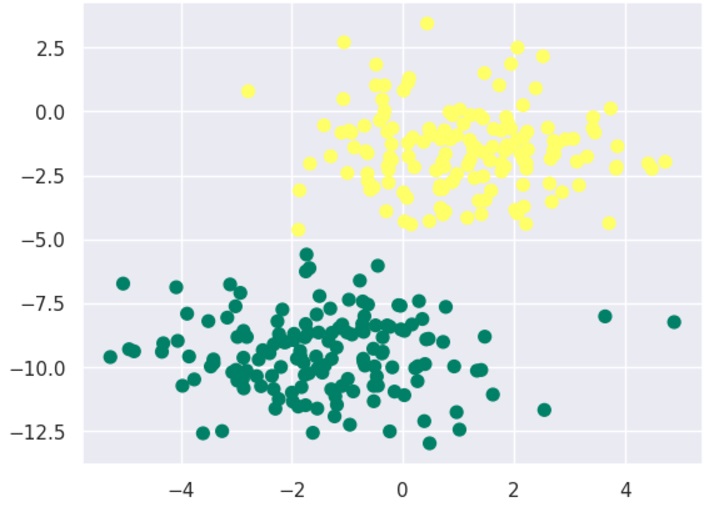
Now, by using make_blobs() function of Scikit learn, we can generate blobs of points with Gaussian distribution as follows −
from sklearn.datasets import make_blobs X, y = make_blobs(300, 2, centers=2, random_state=2, cluster_std=1.5) plt.scatter(X[:, 0], X[:, 1], c=y, s=50, cmap='summer');
Next, for using GaussianNB model, we need to import and make its object as follows −
from sklearn.naive_bayes import GaussianNB model_GNB = GaussianNB() model_GNB.fit(X, y);
Now, we have to do prediction. It can be done after generating some new data as follows −
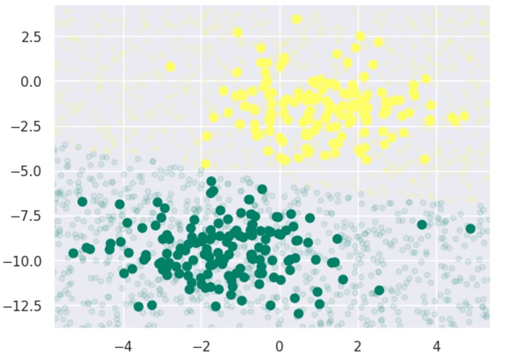
rng = np.random.RandomState(0) Xnew = [-6, -14] + [14, 18] * rng.rand(2000, 2) ynew = model_GNB.predict(Xnew)
Next, we are plotting new data to find its boundaries −
plt.scatter(X[:, 0], X[:, 1], c=y, s=50, cmap='summer') lim = plt.axis() plt.scatter(Xnew[:, 0], Xnew[:, 1], c=ynew, s=20, cmap='summer', alpha=0.1) plt.axis(lim);
Now, with the help of following line of codes, we can find the posterior probabilities of first and second label −
yprob = model_GNB.predict_proba(Xnew) yprob[-10:].round(3)
Output
array([[0.998, 0.002], [1. , 0. ], [0.987, 0.013], [1. , 0. ], [1. , 0. ], [1. , 0. ], [1. , 0. ], [1. , 0. ], [0. , 1. ], [0.986, 0.014]] )
Pros & Cons of Nave Bayes classification
Let's discuss some of the advantages and limitations of Naive Bayes classification algorithm.
Pros
The followings are some pros of using Nave Bayes classifiers −
Nave Bayes classification is easy to implement and fast.
It will converge faster than discriminative models like logistic regression.
It requires less training data.
It is highly scalable in nature, or they scale linearly with the number of predictors and data points.
It can make probabilistic predictions and can handle continuous as well as discrete data.
Nave Bayes classification algorithm can be used for binary as well as multi-class classification problems both.
Cons
The followings are some cons of using Nave Bayes classifiers −
One of the most important cons of Nave Bayes classification is its strong feature independence because in real life it is almost impossible to have a set of features which are completely independent of each other.
Another issue with Nave Bayes classification is its 'zero frequency' which means that if a categorial variable has a category but not being observed in training data set, then Nave Bayes model will assign a zero probability to it and it will be unable to make a prediction.
Applications of Nave Bayes classification
The following are some common applications of Nave Bayes classification −
Real-time prediction − Due to its ease of implementation and fast computation, it can be used to do prediction in real-time.
Multi-class prediction − Nave Bayes classification algorithm can be used to predict posterior probability of multiple classes of target variable.
Text classification − Due to the feature of multi-class prediction, Nave Bayes classification algorithms are well suited for text classification. That is why it is also used to solve problems like spam-filtering and sentiment analysis.
Recommendation system − Along with the algorithms like collaborative filtering, Nave Bayes makes a Recommendation system which can be used to filter unseen information and to predict weather a user would like the given resource or not.