- ML - Home
- ML - Introduction
- ML - Getting Started
- ML - Basic Concepts
- ML - Ecosystem
- ML - Python Libraries
- ML - Applications
- ML - Life Cycle
- ML - Required Skills
- ML - Implementation
- ML - Challenges & Common Issues
- ML - Limitations
- ML - Reallife Examples
- ML - Data Structure
- ML - Mathematics
- ML - Artificial Intelligence
- ML - Neural Networks
- ML - Deep Learning
- ML - Getting Datasets
- ML - Categorical Data
- ML - Data Loading
- ML - Data Understanding
- ML - Data Preparation
- ML - Models
- ML - Supervised Learning
- ML - Unsupervised Learning
- ML - Semi-supervised Learning
- ML - Reinforcement Learning
- ML - Supervised vs. Unsupervised
- Machine Learning Data Visualization
- ML - Data Visualization
- ML - Histograms
- ML - Density Plots
- ML - Box and Whisker Plots
- ML - Correlation Matrix Plots
- ML - Scatter Matrix Plots
- Statistics for Machine Learning
- ML - Statistics
- ML - Mean, Median, Mode
- ML - Standard Deviation
- ML - Percentiles
- ML - Data Distribution
- ML - Skewness and Kurtosis
- ML - Bias and Variance
- ML - Hypothesis
- Regression Analysis In ML
- ML - Regression Analysis
- ML - Linear Regression
- ML - Simple Linear Regression
- ML - Multiple Linear Regression
- ML - Polynomial Regression
- Classification Algorithms In ML
- ML - Classification Algorithms
- ML - Logistic Regression
- ML - K-Nearest Neighbors (KNN)
- ML - Naïve Bayes Algorithm
- ML - Decision Tree Algorithm
- ML - Support Vector Machine
- ML - Random Forest
- ML - Confusion Matrix
- ML - Stochastic Gradient Descent
- Clustering Algorithms In ML
- ML - Clustering Algorithms
- ML - Centroid-Based Clustering
- ML - K-Means Clustering
- ML - K-Medoids Clustering
- ML - Mean-Shift Clustering
- ML - Hierarchical Clustering
- ML - Density-Based Clustering
- ML - DBSCAN Clustering
- ML - OPTICS Clustering
- ML - HDBSCAN Clustering
- ML - BIRCH Clustering
- ML - Affinity Propagation
- ML - Distribution-Based Clustering
- ML - Agglomerative Clustering
- Dimensionality Reduction In ML
- ML - Dimensionality Reduction
- ML - Feature Selection
- ML - Feature Extraction
- ML - Backward Elimination
- ML - Forward Feature Construction
- ML - High Correlation Filter
- ML - Low Variance Filter
- ML - Missing Values Ratio
- ML - Principal Component Analysis
- Reinforcement Learning
- ML - Reinforcement Learning Algorithms
- ML - Exploitation & Exploration
- ML - Q-Learning
- ML - REINFORCE Algorithm
- ML - SARSA Reinforcement Learning
- ML - Actor-critic Method
- ML - Monte Carlo Methods
- ML - Temporal Difference
- Deep Reinforcement Learning
- ML - Deep Reinforcement Learning
- ML - Deep Reinforcement Learning Algorithms
- ML - Deep Q-Networks
- ML - Deep Deterministic Policy Gradient
- ML - Trust Region Methods
- Quantum Machine Learning
- ML - Quantum Machine Learning
- ML - Quantum Machine Learning with Python
- Machine Learning Miscellaneous
- ML - Performance Metrics
- ML - Automatic Workflows
- ML - Boost Model Performance
- ML - Gradient Boosting
- ML - Bootstrap Aggregation (Bagging)
- ML - Cross Validation
- ML - AUC-ROC Curve
- ML - Grid Search
- ML - Data Scaling
- ML - Train and Test
- ML - Association Rules
- ML - Apriori Algorithm
- ML - Gaussian Discriminant Analysis
- ML - Cost Function
- ML - Bayes Theorem
- ML - Precision and Recall
- ML - Adversarial
- ML - Stacking
- ML - Epoch
- ML - Perceptron
- ML - Regularization
- ML - Overfitting
- ML - P-value
- ML - Entropy
- ML - MLOps
- ML - Data Leakage
- ML - Monetizing Machine Learning
- ML - Types of Data
- Machine Learning - Resources
- ML - Quick Guide
- ML - Cheatsheet
- ML - Interview Questions
- ML - Useful Resources
- ML - Discussion
Decision Trees Algorithm in Machine Learning
Decision Tree Algorithm
The decision tree algorithm is a hierarchical tree-based algorithm that is used to classify or predict outcomes based on a set of rules. It works by splitting the data into subsets based on the values of the input features. The algorithm recursively splits the data until it reaches a point where the data in each subset belongs to the same class or has the same value for the target variable. The resulting tree is a set of decision rules that can be used to make predictions or classify new data.
The Decision Tree algorithm works by selecting the best feature to split the data at each node. The best feature is the one that provides the most information gain or the most reduction in entropy. Information gain is a measure of the amount of information gained by splitting the data at a particular feature, while entropy is a measure of the randomness or disorder in the data. The algorithm uses these measures to determine the best feature to split the data at each node.
The example of a binary tree for predicting whether a person is fit or unfit providing various information like age, eating habits and exercise habits, is given below −
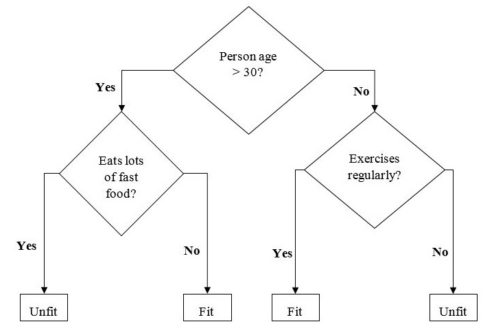
In the above decision tree, the question are decision nodes and final outcomes are leaves.
Types of Decision Tree Algorithm
There are two main types of Decision Tree algorithm −
Classification Tree − A classification tree is used to classify data into different classes or categories. It works by splitting the data into subsets based on the values of the input features and assigning each subset to a different class.
Regression Tree − A regression tree is used to predict numerical values or continuous variables. It works by splitting the data into subsets based on the values of the input features and assigning each subset a numerical value.
Implementing Decision Tree Algorithm
Gini Index
It is the name of the cost function that is used to evaluate the binary splits in the dataset and works with the categorial target variable Success or Failure.
Higher the value of Gini index, higher the homogeneity. A perfect Gini index value is 0 and worst is 0.5 (for 2 class problem). Gini index for a split can be calculated with the help of following steps −
First, calculate Gini index for sub-nodes by using the formula p^2+q^2 , which is the sum of the square of probability for success and failure.
Next, calculate Gini index for split using weighted Gini score of each node of that split.
Classification and Regression Tree (CART) algorithm uses Gini method to generate binary splits.
Split Creation
A split is basically including an attribute in the dataset and a value. We can create a split in dataset with the help of following three parts −
Part1: Calculating Gini Score − We have just discussed this part in the previous section.
Part2: Splitting a dataset − It may be defined as separating a dataset into two lists of rows having index of an attribute and a split value of that attribute. After getting the two groups - right and left, from the dataset, we can calculate the value of split by using Gini score calculated in first part. Split value will decide in which group the attribute will reside.
Part3: Evaluating all splits − Next part after finding Gini score and splitting dataset is the evaluation of all splits. For this purpose, first, we must check every value associated with each attribute as a candidate split. Then we need to find the best possible split by evaluating the cost of the split. The best split will be used as a node in the decision tree.
Building a Tree
As we know that a tree has root node and terminal nodes. After creating the root node, we can build the tree by following two parts −
Part1: Terminal node creation
While creating terminal nodes of decision tree, one important point is to decide when to stop growing tree or creating further terminal nodes. It can be done by using two criteria namely maximum tree depth and minimum node records as follows −
Maximum Tree Depth − As name suggests, this is the maximum number of the nodes in a tree after root node. We must stop adding terminal nodes once a tree reached at maximum depth i.e. once a tree got maximum number of terminal nodes.
Minimum Node Records − It may be defined as the minimum number of training patterns that a given node is responsible for. We must stop adding terminal nodes once tree reached at these minimum node records or below this minimum.
Terminal node is used to make a final prediction.
Part2: Recursive Splitting
As we understood about when to create terminal nodes, now we can start building our tree. Recursive splitting is a method to build the tree. In this method, once a node is created, we can create the child nodes (nodes added to an existing node) recursively on each group of data, generated by splitting the dataset, by calling the same function again and again.
Prediction
After building a decision tree, we need to make a prediction about it. Basically, prediction involves navigating the decision tree with the specifically provided row of data.
We can make a prediction with the help of recursive function, as did above. The same prediction routine is called again with the left or the child right nodes.
Assumptions
The following are some of the assumptions we make while creating decision tree −
While preparing decision trees, the training set is as root node.
Decision tree classifier prefers the features values to be categorical. In case if you want to use continuous values then they must be done discretized prior to model building.
Based on the attributes values, the records are recursively distributed.
Statistical approach will be used to place attributes at any node position i.e.as root node or internal node.
Implementation in Python
Let's implement the Decision Tree algorithm in Python using a popular dataset for classification tasks named Iris dataset. It contains 150 samples of iris flowers, each with four features: sepal length, sepal width, petal length, and petal width. The flowers belong to three classes: setosa, versicolor, and virginica.
First, we will import the necessary libraries and load the dataset −
import numpy as np from sklearn.datasets import load_iris from sklearn.model_selection import train_test_split from sklearn.tree import DecisionTreeClassifier # Load the iris dataset iris = load_iris() # Split the dataset into training and testing sets X_train, X_test, y_train, y_test = train_test_split(iris.data, iris.target, test_size=0.3, random_state=0)
We then create an instance of the Decision Tree classifier and train it on the training set −
# Create a Decision Tree classifier dtc = DecisionTreeClassifier() # Fit the classifier to the training data dtc.fit(X_train, y_train)
We can now use the trained classifier to make predictions on the testing set −
# Make predictions on the testing data y_pred = dtc.predict(X_test)
We can evaluate the performance of the classifier by calculating its accuracy −
# Calculate the accuracy of the classifier accuracy = np.sum(y_pred == y_test) / len(y_test) print("Accuracy:", accuracy) We can visualize the Decision Tree using Matplotlib library −
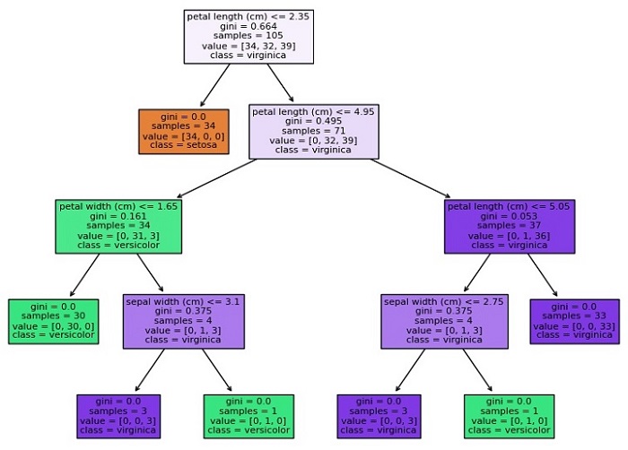
import matplotlib.pyplot as plt from sklearn.tree import plot_tree # Visualize the Decision Tree using Matplotlib plt.figure(figsize=(20,10)) plot_tree(dtc, filled=True, feature_names=iris.feature_names, class_names=iris.target_names) plt.show()
The plot_tree function from the sklearn.tree module can be used to plot the Decision Tree. We can pass in the trained Decision Tree classifier, the filled argument to fill the nodes with color, the feature_names argument to label the features, and the class_names argument to label the target classes. We also specify the figsize argument to set the size of the figure and call the show function to display the plot.
Complete Implementation Example
Given below is the complete implementation example of Decision Tree Classification algorithm in python using the iris dataset −
import numpy as np from sklearn.datasets import load_iris from sklearn.model_selection import train_test_split from sklearn.tree import DecisionTreeClassifier # Load the iris dataset iris = load_iris() # Split the dataset into training and testing sets X_train, X_test, y_train, y_test = train_test_split(iris.data, iris.target, test_size=0.3, random_state=0) # Create a Decision Tree classifier dtc = DecisionTreeClassifier() # Fit the classifier to the training data dtc.fit(X_train, y_train) # Make predictions on the testing data y_pred = dtc.predict(X_test) # Calculate the accuracy of the classifier accuracy = np.sum(y_pred == y_test) / len(y_test) print("Accuracy:", accuracy) # Visualize the Decision Tree using Matplotlib import matplotlib.pyplot as plt from sklearn.tree import plot_tree plt.figure(figsize=(20,10)) plot_tree(dtc, filled=True, feature_names=iris.feature_names, class_names=iris.target_names) plt.show() Output
This will create a plot of the Decision Tree that looks like this −
Accuracy: 0.9777777777777777
As you can see, the plot shows the structure of the Decision Tree, with each node representing a decision based on the value of a feature, and each leaf node representing a class or numerical value. The color of each node indicates the majority class or value of the samples in that node, and the numbers at the bottom indicate the number of samples that reach that node.