SlideShare a Scribd company logo
1 Indian Institute of Technology (ISM), Dhanbad Department of Mining Engineering A group project on COMPUTER AIDED MINE PLANNING Guided by: Dr. Siddharth Agarwal Assistant Professor Department of Mining Engineering Submitted by: Group: DREAM Himanshu Shekhar (17JE003539) Navendu Kumar (17JE003560) Harish Kumar Machra (17JE003549) Ashwini Kumar (17JE003098)
2 CONTENTS: 1. Introduction --------------------------------------------------------------------------------------------3 2. Overall Workflow--------------------------------------------------------------------------------------4 3. Creating a Surpac Geological Database----------------------------------------------------------5 4. Importing drill hole data-----------------------------------------------------------------------------7 5. Display drill hole---------------------------------------------------------------------------------------8 6. Compositing--------------------------------------------------------------------------------------------10 7. Basic statistics------------------------------------------------------------------------------------------11 8. Sectioning and Digitizing of drill hole-------------------------------------------------------------13 9. Validation report of solid----------------------------------------------------------------------------16 10. Variogram modelling of data-----------------------------------------------------------------------17 11. Block modelling and grade estimation in each block using Kriging-----------------------22 12. Pit design and Ramp design-------------------------------------------------------------------------28 13. Results and Conclusion-------------------------------------------------------------------------------32
3 INTRODUCTION: Mine planning: Strength of a building depends on its strength of its foundation. Same is true for mining as well. As the foundation of all mining activity – a mine plan – most accurately reflects the real- time reality of the geological structure in the ground, the process capabilities and the economic unpredictability of demand and commodity markets; which results in a productive, predictable and profitable system within mining structure. To optimize mine profitability, planners and schedulers are under constant pressure to create mine plans that are as accurate as possible and optimize production at all stages, from mine to market. Geo-statistics: Geo-statistics is a branch of statistics focusing on spatial datasets. It is method of predicting probability distributions of ore grades for mining operations. It is intimately related to interpolation methods, but extends far beyond simple interpolation methods. This technique relies on statistical models that are based on random function theory to model the uncertainty associated with spatial estimation and simulation. Surpac: In this project we have used GEOVIA Surpac for studying and further planning of the mine using the data provided by the instructor. GEOVIA Surpac is the world’s most popular geology and mine planning software, supporting open pit and underground operations and exploration projects. Using Surpac, we can visualize an interpolation, lock it in 3-D and then we can bring in all the drilling, all the infrastructure, the development, the headings and know instantly whether we are on track. It also allows us integrate various processes to result a well-designed plan.
4 Overall Workflow Collect field data Make a Blank Database in Surpac Feed the field data in that blank database Display drillholes Sectioning Ore Modelling Compositing Grade Analysis using Histograms Variogram analysis and modelling Block Modelling and reserve estimation Ultimate Pit, Ramp Design and bench Design
5 Creating a Surpac Geological Database: Terminologies: - Geological Database: Geological database is the systematic collection of Drill Hole data. And drill hole data is starting of all the mine project. On the basis of this feasibility study and reserve estimation is done. A geological database consists of a number of tables, each of which contains different types of data. Each table contains a number of fields. Each table also has many records, with each record containing the data fields. Surpac use rational database model. For this project we use three mandatory table and three optional table for the geological database: Mandatory Tables: Collar, Survey, Translation Table (Surpac’s default) Optional Tables: Assay, Geology, Style table (surpac’s default) Collar Table: The information stored in the collar table describes the location of the drill hole collar, the maximum depth of the hole, and whether a linear or curved hole trace will be calculated when retrieving the hole. mandatory fields for collar table: hole_id, y, x, z, max_depth, hole_path Survey Table: The survey table stores the drill hole survey information used to calculate the drill hole trace coordinates. Mandatory fields for survey table: hole_id, depth, dip, azimuth Assay Table: Assay table is an Interval optional table (depth from to depth to) and assay table store information about the concentration of different components in an interval. Mandatory fields for Assay table: hole_id, depth_from, depth_to Optional fields that we have for assay table: percentages of fe, sio2, Al2O3, loi, p in an interval. Geology Table: It is also an Interval optional table. And it stores information about different geology in an interval. And the different geology of the field store as a code (0-10) known as lithocode(lcode). Mandatory fields for the geology table: hole_id, depth_from, depth_to, lcode Steps: Profile of surpac interface set as geological_database 1. Choose Database > Open/New. 2. Enter the name of database, and click Apply 3. Create definition for new database wizard open and click Apply 4. Choose database type as Access and click Apply
6 5. Mandatory table (collar, survey and translation table) already created after the above step. 6. Choose optional table i.e. Assay and Geology add these and define optional as interval 7. After that define all fields for all tables window appear and fill the assay table fields and geological table fields and add variable according to data we have. And click Apply
7 The database is created. The database name appears on the status line to indicate that you are connected to it. Two files have been created: 1. dream_database.mbd The Microsoft Access database which contains the data. 2. dream_ database.ddb The file that Surpac requires to connect to the database. Importing Drill Hole Data: For the importing of drill hole data in a database we have created first we have to connect database. Steps: 1. First, go to Database>import data. 2. Write format file name. Format file name is the name of the header. 3. Click Apply. Dream_database.dsc will created. . dsc is the file extension for a description file. 4. Click Apply. 5. Select the text file for each table. Select load type as insert and update. Click Apply. 6. Extra file also generates during this process with .rej file means rejected file. And all the error generated throughout process were encountered in these files.
8 7. Now all the tables imported and a report file also generated. 8. Now, we can view the imported tables by go to Edit>View tables>Select table name. 9. If we have to edit table then go to Edit>Edit tables>Select table name. 10. We can insert the new data by doing Edit>Insert records>Select table name. 11. And if we want to delete data then Edit>delete>select table name. Display Drill holes: Steps: 1. Firstly, we have to connect the database after that click Display Drillhole. 2. Then define query constraints form will be displayed. 3. Fill the necessary information and click Apply. 4. Then drill holes will be displayed in plan view.
9 Apply styles on dill holes: For the batter visualization and differentiate between the grades. Steps: 1. Go on the menu, and select database. 2. Click database, then click display. 3. Then click drill hole display style. 4. Choose database>display>drill hole display style. 5. And click Apply. 6. After adding all the style for each interval of fe grade do same for lithology also. 7. After that display drill hole for fe. 8. We can see the fe grade also by adding labels, graphs, depth markers. we can also add the cylinder around the drill hole. The radius of cylinder varies accordingly grade value.
10 Compositing: Terminology: Compositing: Compositing is a technique by which assay data are combined to form weighted average or composite grades representative of intervals longer than their own. After core is extracted and logged by the geologist and representative samples are sent out for assaying. Upon receipt, the assays are added to the other geological information such as length, depth, lithology etc. The se individual assay values may represent core lengths of a few inches up to many feet. Steps: 1. Choose Database > Composite > Downhole. 2. Enter the accordingly, and click Apply. Here we took compositing length of 5m. 3. In the report panel we can see the total number of samples, mean, number of boreholes that are processed etc. 4. This string file is generated.
11 5. White string shows the values having sample length greater than or equal to 3.75m. and the Blue string shows the values having sample length less than 3.75m. 6. We can see the statistics of sample data by right click on the string file and click Edit. Basic Statistics: Terminologies: Histogram: A histogram is a bar graph-like representation of data that buckets a range of outcomes into columns along the x-axis. The y-axis represents the number count or percentage of occurrences in the data for each column and can be used to visualize data distributions. Outlier: An outlier is an observation that lies an abnormal distance from other values in a random sample from a population. In a sense, this definition leaves it up to the analyst (or a consensus process) to decide what will be considered abnormal. Steps: 1. For opening the basic statistics window in surpac click Database>Analysis>Basic statistics window.
12 2. Click file>Load data from string file. select the string file. and Click Apply. And histogram will appear with cumulative frequency curve. 3. We can only see the histogram by click display>histogram. And save histogram by clicking save icon. 4. Normal distribution curve of data made by clicking on Display>normal distribution curve.
13 5. Above one is negatively skewed normal distribution curve. And have outliers. So, we have to remove these outliers for this click File tool>string Maths. A string math form will appear. Select the compositing string file and enter the output file name. and write down Expression properly. 6. After removing outliers, the negatively skewed normal distribution curve now become slightly normal curve. 7. This compositing file does not contain any outliers hence it will be used in Variogram modelling. Sectioning and Digitising of Drill Holes: Terminologies: Sectioning: Sectioning is the process of creating a mirror image of the drill holes when cut through by a plane. Digitizing: digitising is the act of outlining the ore terrain or mineralization. We will use this to define the extent of the ore body based on the direction and length of drill holes. Steps involve in sectioning: 1. Firstly, we have to connect the database then, Display the drillholes after that 2. Click Sections>Define
14 3. Define slicing planes width window will open define the section definition method, enter distance forward of plane, distance backward of plane and section by interval. 4. Click Apply 5. After that one section of drill hole appear. 6. For viewing next section go to sections>Next. And we can see the previous section also sections>Previous. Steps involve in Digitizing: For digitizing already define section we have to follow these steps: 1. Click create>digitise>New point 2. Then digitise end points of ore zone by clicking the right click and choose the point and covers all the drill hole boundaries. 3. After one section digitization complete go to section>next and do same for the next section of drill holes. 4. After completing of all the sections save the string file by go to File>save>string.
15 5. Open the string file and for the solid go to solid>Triangulation and for the outer segment choose Inside a segment and for the rest choose Between the segment option. After completing this Save the file. 6. We can calculate the volume of this solid or ore zone by clicking Surfaces>volume>Report volume of solids
16 Validation Report of solid: Validation report of solid shows us that whether proper formation of solid is done or not. It is manly depending on the proper triangulation. Steps: 1. Click Solids>Validation>Validate object/trisolation 2. Enter Report file name, object range, Trisolation Range and click Apply 3. Validation report will generate 4. If it shows invalid in that case, we have to repair solid by clicking on Solids>Validation>Repair solid.
17 Variogram modelling of the data: Terminologies: Variogram: Variogram is a graph of sample difference (variance) against distance (lag). And it shows how data values change over distance and direction. It has various specific terms is used such as Nugget, Sill, Range etc. A basic variogram: Nugget: Nugget is the different in value of samples taken at a separation distance of zero. This difference is called the “nugget”, also abbreviated as “c(0)”. Sill: Sill is the value at which the variogram levels off or flattens out. Difference between sample values continuous increase until at some point the greatest difference is attained, represent by flat portion of the variogram. Represent as “C”.
18 Total sill: Total sill is the nugget to sill ratio. (nugget / (nugget + sill) Range: Range is the maximum distance at which the sill attained. Sometime represented as “A”. After the range there is no relationship between data. Isotropy Data: Isotropy means the values measured in different direction are same. Anisotropy Data: Anisotropy means having the difference value in different direction. Omnidirectional variogram: In omnidirectional variogram, sample pairs are selected based only on their separation distance. Directional variogram: In this, sample pairs are selected based on a particular direction or orientation. Variogram analysis consists of the experimental variogram calculated from the data and the variogram model fitted to the data. Steps: 1. For opening of variogram window click Block model>Geostatistics>Variogram modelling. 2. For the experiment variogram first we should have Compositing String file for fe without any outlier. So, we have to remove all the outlier before the variogram analysis. 3. Now for the experiment variogram from data click File>New>String file variogram. 4. After that variogram calculation window will appear. Fill all the required options accordingly. We choose firstly Lag distance 10, maximum distance ( it is around the half of the distance between the outer segment of the ore or half of total extended ore) is around 625 m. In this we also get advance option for variogram calculation in which we can add Geographical constrain and properties of Lag slider. 5. After filling all the details click Apply.
19 6. After that an experimental variogram appear with lag distance 10. We can change the lag distance by click on right side of Lag slider. We changed at 20 for better representation. If we took the lag distance low then no of pairs at each lag distance increase. 7. There are different Variogram Model such as Spherical, Exponential, Gaussian, Hole Effect. So, try each one for best fitting. Here Spherical type of variogram used for modelling because it gave the best fit curve on experimental variogram. 8. Now, we have to fit variogram model on this experiment variogram for the calculation of different attributes of it. So, for that click Variogram>model or we can change the variogram model by click on variogram model type. With the help of variogram structure try to fit model on the experiment variogram. At least 3-4 points of model should be lies on experimental variogram. 9. And, we can see the number of pair for each lag distance by click on display/hide number of pairs.
20 10. When we best fit the variogram model on the experimental variogram we see the values of various parameters on the right side of variogram. In this case, Nugget value is around 2, sill around 50, and the range is around 130. 11. For the report of variogram click Variogram>Report. And enter the file name and click Apply. Report will generate in not file. 12. There is various Experimental variogram type i.e. standard, Normalised, Logarithmic, General Relative and Pairwise Relative. So, Choose accordingly. We choose standard for this. 13. Now save the variogram model and experimental model by click save the experimental variogram and model. 14. There are various options such as add model, delete model, add structure, Delete structure, validation.
21 15. so here is various model fitted on the experimental variogram Exponential Model: Gaussian: Hole effect: 16. Now, similar steps were taken for creating a variogram for the gangue (combined value of SiO2+ Al2O3+P) from gangue composite string created. Use the compositing file which do not have any outlier, so we created a spherical variogram directly and fit the model accordingly. And find out all the Attributes for them.
22 Block Modelling and Grade estimation in each Block using Krigging Terminologies: - Block Modelling – Once the ore model is made, there is a need to divide the entire ore body into number of blocks, this process is called Block Modelling. Block size- For block modelling there is a need to estimate the size of each block. As a rule of thumb, the minimum size of the block should not be less than ¼ of average drill hole interval, say 25m blocks for a 100 meters drilling grid. The height of the block is often that of the bench height for mining. For this project the Block size of l*b*h= 25*25*10 was taken because the drilling grid was of 100 m and the bench height is decided to be of 10m. Grade Estimation- The blocks formed initially do not contain grades. So, in order to assign grades in each block there are some methods like IDW (Inverse distance weighting, Krigging etc.) which need to be followed. The tonnage of each block can be easily found from the block volume and the tonnage factor. The blocks are considered as point values rather than as volumes. If the block is divided into a mesh of smaller blocks, the calculation would be made for each sub-block and the results summed. Hughes & Davey (1979) has indicated that the difference between the point and volume approach is small. Choosing the Estimation Technique- Surpac has some in-buit estimation techniques like Inverse Distance, Ordinary Krigging, Simple krigging. Based on our geo-spatial and geostatistical knowledge we have to choose from them. Ordinary Krigging is the most suitable and widely accepted estimation technique as it takes into account if there is a spatially correlated distance or directional bias in the data. For this project Ordinary Krigging was used. Work flow Creating Blank Block Model Adding Attributes to Block Model Estimating Grade Values to each block Adding Constraints to block Model Block Model Reporting
23 Steps: Creating Blank block model. 1. Open ore model.dtm 2. Click Display > 3D Grids and note down the approx. extents of the ore body. For this project Northing was found to be in the range [-900 to 500], Easting in the range [-300 to 500], Elevation in the range [600 to 900]. (all values in meter) 3. Click Block Model > Block Model > New/Open. 4. A ‘Select Model’ dialogue box appears. Enter Model Name, say block_model_1. Click Apply. Then again, a dialogue box appears, Click Apply. 5. ‘Creating new block model definition’ Window appears. Enter the Coordinate extents of X, Y, Z which has been found in Step-2. Coordinate Extents can also be input from the Sectioning string file. Enter block size which has been decided earlier. In Sub blocking choose Standard and Minimum block size of 6.25,6.25,2.5. Click Apply.
24 6. Model Confirmation window appears. Click Create Model. 7. A blank Model has been created and can be displayed by clicking on block_model_1 and on then on Display. A Draw block model dialogue box appears click Apply. 8. Block model is displayed. Adding attributes to the block model 1. Click Block Model> Attributes> New. An Add attribute window appears.Fill the attribute name, type, decimals, Background Value, Description/Expression. Click on Apply. 2. Attribute with name ‘fe’ is created. Estimating grade values to each block 1. Click Block model> Estimation> Ordinary Krigging 2. A Dialogue box Select attributes to model appears. From the drop down choose ‘fe’. 3. Estimation Attributes window appears click apply. Data Source Specifications window appears. In string file location select the composite string file which we have created. Click Apply. For the estimation process we need to feed the values of fe grade at those points which are already known. In our case which is in the form of composite string file.
25 4. A window of Search parameters appears. In this window we have to basically specify the extents up to which the grades are influencing or are corelated. Maximum search radius and maximum vertical search radius depends on the range of variogram model in case of krigging. This precisely explains that up-to how much distance the grades are having their influence. In this particular case the range of the variogram model was around 130. Maximum search radius- 130 Maximum Vertical search radius- 130 Click Apply. .
26 5. Krigging Parameters window opens. In the variogram file name Insert the variogram model created. In number of discretisation point fill X=3, Y=3, Z=3. This basically denotes the direction in which the grades are having their influence. If a greater number of points are selected it will take more time to estimate but will give better estimation. Write the report file name and format. Click Apply. 6. The grades have been applied to each block. To see the grade of a particular block. Click Block Model> Attributes> View attributes of one block. Then click on the block of which you wish to see the grade value. Adding Constraints to Block Model: Constraints are added to constrain our block model to a particular value, blocks or DTM. 1. Click on Block Model> Constraints> New Constraints file. 2. In the add constraints window Select the constraint type then select the file under which we have to constrain the block model. Click Add and then Apply Block Model Reporting Used to report the whole block model. 1. Choose Block Model> Report. 2. Enter the Output report file name and click Apply. 3. Block Model report window opens. In report attributes select the attributes which we have to report. In this case fe was chosen. If we want our report to contain weight then specific gravity should be provided in the density arrangement. Groupby attributes is used to subgroups the different attributes. In this case the fe attribute was further divided into 0- 47.5, 47.5-57.5, 57.5-999 and for Z value 600-700,700-800,800-900. Click Apply.
27 4. Enter constraints window appears. Select 3DM as constraint type and Ore_model.dtm as the constraint file. This will constraint the report which is going to be generated within that ore model solid. Click Apply. 5. A notepad file containing report appears. This file shows the different values of tonnage, volume for different grades of ore.
28 Pit design and Ramp design: Terminologies- Bench Height- The vertical distance between crest and toe of a bench. Mainly dependent on size and type of equipment used in the mine. For this project we are designing for Shovel and Dumper combination. With maximum height of the shovel being 10m. So, Bench Height is also being taken as 10m in accordance with MMR. Bench Face Angle- The bench face angle can vary considerably with rock characteristics, face orientation and blasting practices. In most hard rock pits, it varies from about 55◦ to 80◦. A typical initial design value may be 65 – 70 degree. For this project we have selected a Bench Face Angle of 55. Ramp width- The width of the road should allow enough room for the required number of lanes and all the associated safety and drainage features. For this project we have designed both single lane and double lane haul road with width 14m and 28 m respectively. Ramp Gradient- Depends on the gradeability of the HEMMs and the regulation of that country. For this project Ramp Gradient has been taken as 1 in 16. Switchbacks- Generally switchbacks should be avoided in a pit because it tends to slow down traffic, cause greater tire wear, cause various maintenance problems etc. But sometimes it becomes very necessary to provide switchbacks in the cases like for a gently sloping ore contact which provides room to work in switchbacks at little stripping cost. Work Flow Making of Ultimate Pit Design of Ramp Design of Bench by Bench Height Design of Bench by berm width Creating of DTM from Pit Layout
29 Making of Ultimate Pit Generally, designing of Ramp is a bottom to top process. So, firstly we have to make ultimate pit string file. Number of Ultimate pits depends on the orientation of the block model and on the intuition of the mine designer. Generally, it is better to have several smaller pits rather than one large pit in order to support mine economics. For this project, after investigating the ore body orientation we decided to make 3 pits at RLs of about 650,725,753 so that the stripping ratio also should not unnecessarily increase. Ultimate pit: 1. Open the ore model DTM file. 2. Get the plan view of DTM by clicking on icon. 3. Click on digitise points using mouse and make outlines around the parts of the ore body in which we have to make the individual pits. 4. Once the making of ultimate pits are finished. Adjust the elevation of string files thus created in the section view and by using Edit>String> Move option. It will be as shown in the figure. 5. Save this string file by clicking on the icon. Design of Ramps: 1. Click on the angle icon , then a set the design gradient window opens. Fill the Bench face angle. For our case we had decided it to be 55. 2. Go to Design>Pit Design>New Ramp. Then select the ramp starting points in the bottom most pit. 3. And then define the ramp properties in the shortcut menu of Define a new ramp 4. Ramp properties are: ramp name, ramp string, ramp type, ramp width, ramp gradient, gradient method, berm taper distance, and switchback angle and inner radius.
30 5.And then click apply. A ramp has been defined. Design of Benches: 6. Click Design> Expand Segment > By Bench Height. 7. Select the segment which need to be expanded. 8. Then enter the Bench Height which has been earlier decided, in the pop-up window. 9. Click Apply. Design of Berms: 10. Design> Expand Segment> By Berm width. 11. Enter the Berm width, Gradient of the berm (depend on the make of water in the mine) in the ‘Expand segment by berm width’ window and then click Apply. Continue the above process from 1-10 till we cover the whole ore body. Creating of DTM from the Pit layout 1. Click on Surfaces> Create DTM from Layer 2. Give object Id which displays the colour and uncheck the break line test. Click Apply. 3. DTM of the ultimate pit is generated.
31 Ultimate pit with the Block Model
32 Results and Conclusion: Extents of Ore Body Minimum Maximum X -224.113 425.544 Y -850 450 Z 425.544 425.544 Volume, mass and average grade The average grade of Fe as estimated by Ordinary Krigging method was 60.422 and the total tonnage of Ore estimated was 2.35*108 tonnes. (Sp. Gravity of 5.5 was used).
33 Pit Design: Assumptions: 1. Shovel- Dumper combination to be deployed. 2. Electrical Rope Shovel with maximum digging height= 10,300 mm= 10.3 m 3. Komatsu 100 tonne dumpers with width= 4663.2 mm = 4.6 m Based on these assumptions and keeping the Metal Mines Regulations in account. The following pit design parameters had been selected Bench Height=10m Ramp Width= 14 m Ramp Gradient= 1:16 Berm Width= 5m. Final View of the pit.

More Related Content

What's hot (20)

Open pit mining
Open pit miningOpen pit mining
Open pit mining
Prof. A.Balasubramanian
 
Shrinkage and Vertical Crater Retreat Stoping
Shrinkage and Vertical Crater Retreat StopingShrinkage and Vertical Crater Retreat Stoping
Shrinkage and Vertical Crater Retreat Stoping
Geology Department, Faculty of Science, Tanta University
 
Mining geology an overview
Mining geology an overviewMining geology an overview
Mining geology an overview
Mrinmoy Chakraborty
 
Surface mining planning and design of open pit mining
Surface mining planning and design of open pit miningSurface mining planning and design of open pit mining
Surface mining planning and design of open pit mining
Geology Department, Faculty of Science, Tanta University
 
Introduction to Seismic Method
Introduction to Seismic Method Introduction to Seismic Method
Introduction to Seismic Method
Ahmed Younhais Tariq
 
Room & Pillar Mining Method
Room & Pillar Mining MethodRoom & Pillar Mining Method
Room & Pillar Mining Method
Ayon Saha
 
2 surface mine planning
2 surface mine planning2 surface mine planning
2 surface mine planning
UET Peshawar
 
Cut and Fill mining
Cut and Fill miningCut and Fill mining
Cut and Fill mining
National Institute of Technology, Rourkela
 
Mine scheduling process
Mine scheduling processMine scheduling process
Mine scheduling process
VR M
 
Reserve Estimation Using DATAMINE software
Reserve Estimation Using DATAMINE softwareReserve Estimation Using DATAMINE software
Reserve Estimation Using DATAMINE software
Sushant Kumar
 
Mine planning
Mine planning Mine planning
Mine planning
TarunKumar1052
 
Caving Underground Mining Methods (longwall, Sublevel caving, & Block caving)
Caving Underground Mining Methods (longwall, Sublevel caving, & Block caving)Caving Underground Mining Methods (longwall, Sublevel caving, & Block caving)
Caving Underground Mining Methods (longwall, Sublevel caving, & Block caving)
Geology Department, Faculty of Science, Tanta University
 
Core Concepts Mining Cycle
Core Concepts Mining CycleCore Concepts Mining Cycle
Core Concepts Mining Cycle
Mining Matters
 
Subsidence
SubsidenceSubsidence
Subsidence
Arpit Baderiya
 
Drilling
Drilling Drilling
Drilling
PRAMODA G
 
Underground mining method
Underground mining methodUnderground mining method
Underground mining method
Safdar Ali
 
Geomodelling, resource & reserve estimation using mining software
Geomodelling, resource & reserve estimation using mining softwareGeomodelling, resource & reserve estimation using mining software
Geomodelling, resource & reserve estimation using mining software
Chandra Bose
 
Sublevel open stopping assignment
Sublevel open stopping assignmentSublevel open stopping assignment
Sublevel open stopping assignment
virendrasuryawanshi
 
Pillar design in coal mines
Pillar design in coal minesPillar design in coal mines
Pillar design in coal mines
Ulimella Siva Sankar
 
Underground mining system
Underground mining systemUnderground mining system
Underground mining system
Srimontorumpa
 
Room & Pillar Mining Method
Room & Pillar Mining MethodRoom & Pillar Mining Method
Room & Pillar Mining Method
Ayon Saha
 
2 surface mine planning
2 surface mine planning2 surface mine planning
2 surface mine planning
UET Peshawar
 
Mine scheduling process
Mine scheduling processMine scheduling process
Mine scheduling process
VR M
 
Reserve Estimation Using DATAMINE software
Reserve Estimation Using DATAMINE softwareReserve Estimation Using DATAMINE software
Reserve Estimation Using DATAMINE software
Sushant Kumar
 
Core Concepts Mining Cycle
Core Concepts Mining CycleCore Concepts Mining Cycle
Core Concepts Mining Cycle
Mining Matters
 
Underground mining method
Underground mining methodUnderground mining method
Underground mining method
Safdar Ali
 
Geomodelling, resource & reserve estimation using mining software
Geomodelling, resource & reserve estimation using mining softwareGeomodelling, resource & reserve estimation using mining software
Geomodelling, resource & reserve estimation using mining software
Chandra Bose
 
Sublevel open stopping assignment
Sublevel open stopping assignmentSublevel open stopping assignment
Sublevel open stopping assignment
virendrasuryawanshi
 
Underground mining system
Underground mining systemUnderground mining system
Underground mining system
Srimontorumpa
 

Similar to Resource estimation using Surpac software in mining (20)

3.- Integrating environmental data in ModestR (Version ModestR v5.3 or higher)
3.- Integrating environmental data in ModestR (Version ModestR v5.3 or higher) 3.- Integrating environmental data in ModestR (Version ModestR v5.3 or higher)
3.- Integrating environmental data in ModestR (Version ModestR v5.3 or higher)
modestrsoftware
 
References1. HCS 2010 online manuals.2. Data Data provi.docx
References1. HCS 2010 online manuals.2. Data Data provi.docxReferences1. HCS 2010 online manuals.2. Data Data provi.docx
References1. HCS 2010 online manuals.2. Data Data provi.docx
debishakespeare
 
Software Development for Well Planning
Software Development for Well PlanningSoftware Development for Well Planning
Software Development for Well Planning
International journal of scientific and technical research in engineering (IJSTRE)
 
Watershed Delineation in ArcGIS
Watershed Delineation in ArcGISWatershed Delineation in ArcGIS
Watershed Delineation in ArcGIS
Arthur Green
 
HFSS MICROSTRIP PATCH ANTENNA- ANALYSIS AND DESIGN
HFSS MICROSTRIP PATCH ANTENNA- ANALYSIS AND DESIGNHFSS MICROSTRIP PATCH ANTENNA- ANALYSIS AND DESIGN
HFSS MICROSTRIP PATCH ANTENNA- ANALYSIS AND DESIGN
Shivashu Awasthi
 
GeoServer Orientation
GeoServer OrientationGeoServer Orientation
GeoServer Orientation
Jody Garnett
 
2. Develop a MapReduce program to calculate the frequency of a given word in ...
2. Develop a MapReduce program to calculate the frequency of a given word in ...2. Develop a MapReduce program to calculate the frequency of a given word in ...
2. Develop a MapReduce program to calculate the frequency of a given word in ...
Prof. Maulik Trivedi
 
Unit I - introduction to r language 2.pptx
Unit I - introduction to r language 2.pptxUnit I - introduction to r language 2.pptx
Unit I - introduction to r language 2.pptx
SreeLaya9
 
Watershed Delineation Using ArcMap
Watershed Delineation Using ArcMapWatershed Delineation Using ArcMap
Watershed Delineation Using ArcMap
Arthur Green
 
Unit 2 - Data Manipulation with R.pptx
Unit 2 - Data Manipulation with R.pptxUnit 2 - Data Manipulation with R.pptx
Unit 2 - Data Manipulation with R.pptx
Malla Reddy University
 
How to empower community by using GIS lecture 2
How to empower community by using GIS lecture 2How to empower community by using GIS lecture 2
How to empower community by using GIS lecture 2
wang yaohui
 
EN1320 Module 2 Lab 2.1Capturing the Reader’s InterestSelec.docx
EN1320 Module 2 Lab 2.1Capturing the Reader’s InterestSelec.docxEN1320 Module 2 Lab 2.1Capturing the Reader’s InterestSelec.docx
EN1320 Module 2 Lab 2.1Capturing the Reader’s InterestSelec.docx
YASHU40
 
Week 4 Project - STAT 3001Student Name Type your name here.docx
Week 4 Project - STAT 3001Student Name Type your name here.docxWeek 4 Project - STAT 3001Student Name Type your name here.docx
Week 4 Project - STAT 3001Student Name Type your name here.docx
melbruce90096
 
Optimization of workload prediction based on map reduce frame work in a cloud...
Optimization of workload prediction based on map reduce frame work in a cloud...Optimization of workload prediction based on map reduce frame work in a cloud...
Optimization of workload prediction based on map reduce frame work in a cloud...
eSAT Publishing House
 
Optimization of workload prediction based on map reduce frame work in a cloud...
Optimization of workload prediction based on map reduce frame work in a cloud...Optimization of workload prediction based on map reduce frame work in a cloud...
Optimization of workload prediction based on map reduce frame work in a cloud...
eSAT Journals
 
Tictac
TictacTictac
Tictac
Upendra Sengar
 
Mapreduce Algorithms
Mapreduce AlgorithmsMapreduce Algorithms
Mapreduce Algorithms
Amund Tveit
 
Jaspersoft and Clarity PPM - Advanced Reporting with Data Warehouse
Jaspersoft and Clarity PPM - Advanced Reporting with Data WarehouseJaspersoft and Clarity PPM - Advanced Reporting with Data Warehouse
Jaspersoft and Clarity PPM - Advanced Reporting with Data Warehouse
Thiago Bottoni
 
Week 2 Project - STAT 3001Student Name Type your name here.docx
Week 2 Project - STAT 3001Student Name Type your name here.docxWeek 2 Project - STAT 3001Student Name Type your name here.docx
Week 2 Project - STAT 3001Student Name Type your name here.docx
cockekeshia
 
AgilentHPLC_SOP_Base_1_InfinitySeries.pptx
AgilentHPLC_SOP_Base_1_InfinitySeries.pptxAgilentHPLC_SOP_Base_1_InfinitySeries.pptx
AgilentHPLC_SOP_Base_1_InfinitySeries.pptx
SubhrajitRoy19
 
3.- Integrating environmental data in ModestR (Version ModestR v5.3 or higher)
3.- Integrating environmental data in ModestR (Version ModestR v5.3 or higher) 3.- Integrating environmental data in ModestR (Version ModestR v5.3 or higher)
3.- Integrating environmental data in ModestR (Version ModestR v5.3 or higher)
modestrsoftware
 
References1. HCS 2010 online manuals.2. Data Data provi.docx
References1. HCS 2010 online manuals.2. Data Data provi.docxReferences1. HCS 2010 online manuals.2. Data Data provi.docx
References1. HCS 2010 online manuals.2. Data Data provi.docx
debishakespeare
 
Watershed Delineation in ArcGIS
Watershed Delineation in ArcGISWatershed Delineation in ArcGIS
Watershed Delineation in ArcGIS
Arthur Green
 
HFSS MICROSTRIP PATCH ANTENNA- ANALYSIS AND DESIGN
HFSS MICROSTRIP PATCH ANTENNA- ANALYSIS AND DESIGNHFSS MICROSTRIP PATCH ANTENNA- ANALYSIS AND DESIGN
HFSS MICROSTRIP PATCH ANTENNA- ANALYSIS AND DESIGN
Shivashu Awasthi
 
GeoServer Orientation
GeoServer OrientationGeoServer Orientation
GeoServer Orientation
Jody Garnett
 
2. Develop a MapReduce program to calculate the frequency of a given word in ...
2. Develop a MapReduce program to calculate the frequency of a given word in ...2. Develop a MapReduce program to calculate the frequency of a given word in ...
2. Develop a MapReduce program to calculate the frequency of a given word in ...
Prof. Maulik Trivedi
 
Unit I - introduction to r language 2.pptx
Unit I - introduction to r language 2.pptxUnit I - introduction to r language 2.pptx
Unit I - introduction to r language 2.pptx
SreeLaya9
 
Watershed Delineation Using ArcMap
Watershed Delineation Using ArcMapWatershed Delineation Using ArcMap
Watershed Delineation Using ArcMap
Arthur Green
 
Unit 2 - Data Manipulation with R.pptx
Unit 2 - Data Manipulation with R.pptxUnit 2 - Data Manipulation with R.pptx
Unit 2 - Data Manipulation with R.pptx
Malla Reddy University
 
How to empower community by using GIS lecture 2
How to empower community by using GIS lecture 2How to empower community by using GIS lecture 2
How to empower community by using GIS lecture 2
wang yaohui
 
EN1320 Module 2 Lab 2.1Capturing the Reader’s InterestSelec.docx
EN1320 Module 2 Lab 2.1Capturing the Reader’s InterestSelec.docxEN1320 Module 2 Lab 2.1Capturing the Reader’s InterestSelec.docx
EN1320 Module 2 Lab 2.1Capturing the Reader’s InterestSelec.docx
YASHU40
 
Week 4 Project - STAT 3001Student Name Type your name here.docx
Week 4 Project - STAT 3001Student Name Type your name here.docxWeek 4 Project - STAT 3001Student Name Type your name here.docx
Week 4 Project - STAT 3001Student Name Type your name here.docx
melbruce90096
 
Optimization of workload prediction based on map reduce frame work in a cloud...
Optimization of workload prediction based on map reduce frame work in a cloud...Optimization of workload prediction based on map reduce frame work in a cloud...
Optimization of workload prediction based on map reduce frame work in a cloud...
eSAT Publishing House
 
Optimization of workload prediction based on map reduce frame work in a cloud...
Optimization of workload prediction based on map reduce frame work in a cloud...Optimization of workload prediction based on map reduce frame work in a cloud...
Optimization of workload prediction based on map reduce frame work in a cloud...
eSAT Journals
 
Mapreduce Algorithms
Mapreduce AlgorithmsMapreduce Algorithms
Mapreduce Algorithms
Amund Tveit
 
Jaspersoft and Clarity PPM - Advanced Reporting with Data Warehouse
Jaspersoft and Clarity PPM - Advanced Reporting with Data WarehouseJaspersoft and Clarity PPM - Advanced Reporting with Data Warehouse
Jaspersoft and Clarity PPM - Advanced Reporting with Data Warehouse
Thiago Bottoni
 
Week 2 Project - STAT 3001Student Name Type your name here.docx
Week 2 Project - STAT 3001Student Name Type your name here.docxWeek 2 Project - STAT 3001Student Name Type your name here.docx
Week 2 Project - STAT 3001Student Name Type your name here.docx
cockekeshia
 
AgilentHPLC_SOP_Base_1_InfinitySeries.pptx
AgilentHPLC_SOP_Base_1_InfinitySeries.pptxAgilentHPLC_SOP_Base_1_InfinitySeries.pptx
AgilentHPLC_SOP_Base_1_InfinitySeries.pptx
SubhrajitRoy19
 

Recently uploaded (20)

EXAFS for Structural Characterization, Extended X-ray Absorption Fine Structure
EXAFS for Structural Characterization, Extended X-ray Absorption Fine StructureEXAFS for Structural Characterization, Extended X-ray Absorption Fine Structure
EXAFS for Structural Characterization, Extended X-ray Absorption Fine Structure
KikiRezkiLestari1
 
NMR Notes_240102_162930 log geophysics.pdf
NMR Notes_240102_162930 log geophysics.pdfNMR Notes_240102_162930 log geophysics.pdf
NMR Notes_240102_162930 log geophysics.pdf
ak930123aman
 
ELECTROCHEMISTRY FOR 1ST YEAR CHEMISTRY.pdf
ELECTROCHEMISTRY FOR 1ST YEAR CHEMISTRY.pdfELECTROCHEMISTRY FOR 1ST YEAR CHEMISTRY.pdf
ELECTROCHEMISTRY FOR 1ST YEAR CHEMISTRY.pdf
AshikaAgarwal6
 
The_Evolution_of_Software_Configuration_Management.pdf
The_Evolution_of_Software_Configuration_Management.pdfThe_Evolution_of_Software_Configuration_Management.pdf
The_Evolution_of_Software_Configuration_Management.pdf
vemiri6305
 
Software Screen Universal Snubber machine (2).pptx
Software Screen Universal Snubber machine (2).pptxSoftware Screen Universal Snubber machine (2).pptx
Software Screen Universal Snubber machine (2).pptx
Neometrix_Engineering_Pvt_Ltd
 
This research study focuses on flood hazard analysis in the Chbar Ampov distr...
This research study focuses on flood hazard analysis in the Chbar Ampov distr...This research study focuses on flood hazard analysis in the Chbar Ampov distr...
This research study focuses on flood hazard analysis in the Chbar Ampov distr...
Panha NUTH
 
Experimental techniques and instrumentation
Experimental techniques and instrumentationExperimental techniques and instrumentation
Experimental techniques and instrumentation
drharipriya42
 
Low cost Housing and Apartment Literature review
Low cost Housing and Apartment Literature reviewLow cost Housing and Apartment Literature review
Low cost Housing and Apartment Literature review
sadikshyaripple
 
Basic Python Programs, Python Fundamentals.pptx
Basic Python Programs, Python Fundamentals.pptxBasic Python Programs, Python Fundamentals.pptx
Basic Python Programs, Python Fundamentals.pptx
SrinivasGopalan2
 
ExcitonSummary, Wannier Mott and Frenkel Excitons
ExcitonSummary, Wannier Mott and Frenkel ExcitonsExcitonSummary, Wannier Mott and Frenkel Excitons
ExcitonSummary, Wannier Mott and Frenkel Excitons
ralagaadedayo
 
Cryptography 3 Cryptography 3 Cryptography 3
Cryptography 3 Cryptography 3 Cryptography 3Cryptography 3 Cryptography 3 Cryptography 3
Cryptography 3 Cryptography 3 Cryptography 3
AhmedSaeed115917
 
call for Papers - 6th International Conference on Natural Language Computing ...
call for Papers - 6th International Conference on Natural Language Computing ...call for Papers - 6th International Conference on Natural Language Computing ...
call for Papers - 6th International Conference on Natural Language Computing ...
CSEIJJournal
 
Best of Two Avg, Python Program To Find Average of Two Numbers.pptx
Best of Two Avg, Python Program To Find Average of Two Numbers.pptxBest of Two Avg, Python Program To Find Average of Two Numbers.pptx
Best of Two Avg, Python Program To Find Average of Two Numbers.pptx
SrinivasGopalan2
 
Anti-Riot_Drone_Phase-0(2)[1] major project.pptx
Anti-Riot_Drone_Phase-0(2)[1] major project.pptxAnti-Riot_Drone_Phase-0(2)[1] major project.pptx
Anti-Riot_Drone_Phase-0(2)[1] major project.pptx
neerajprajwal
 
Music player case study using C++ and others
Music player case study using C++ and othersMusic player case study using C++ and others
Music player case study using C++ and others
simonoct8
 
Safety pdf , this is tha very important & very useful in a safety
Safety pdf , this is tha very important & very useful in a safetySafety pdf , this is tha very important & very useful in a safety
Safety pdf , this is tha very important & very useful in a safety
arpit987dwivedi
 
WORK AT HEIGHT TRAINING WORK AT HEIGHT TRAINING.pptx
WORK AT HEIGHT TRAINING WORK AT HEIGHT TRAINING.pptxWORK AT HEIGHT TRAINING WORK AT HEIGHT TRAINING.pptx
WORK AT HEIGHT TRAINING WORK AT HEIGHT TRAINING.pptx
ahnngomaa
 
PRIZ Academy - Root Cause Analysis (RCA) Quality Assurance with PRIZ .pdf
PRIZ Academy - Root Cause Analysis (RCA) Quality Assurance with PRIZ .pdfPRIZ Academy - Root Cause Analysis (RCA) Quality Assurance with PRIZ .pdf
PRIZ Academy - Root Cause Analysis (RCA) Quality Assurance with PRIZ .pdf
PRIZ Guru
 
Transportation Design at Ajeenkya DY Patil Univeristy
Transportation Design at Ajeenkya DY Patil UniveristyTransportation Design at Ajeenkya DY Patil Univeristy
Transportation Design at Ajeenkya DY Patil Univeristy
sourabhmore19
 
Mohamed Ahmed Ali Ahmed Ali Katheer CV new update
Mohamed Ahmed Ali Ahmed Ali Katheer CV new updateMohamed Ahmed Ali Ahmed Ali Katheer CV new update
Mohamed Ahmed Ali Ahmed Ali Katheer CV new update
AhmedKatheer1
 
EXAFS for Structural Characterization, Extended X-ray Absorption Fine Structure
EXAFS for Structural Characterization, Extended X-ray Absorption Fine StructureEXAFS for Structural Characterization, Extended X-ray Absorption Fine Structure
EXAFS for Structural Characterization, Extended X-ray Absorption Fine Structure
KikiRezkiLestari1
 
NMR Notes_240102_162930 log geophysics.pdf
NMR Notes_240102_162930 log geophysics.pdfNMR Notes_240102_162930 log geophysics.pdf
NMR Notes_240102_162930 log geophysics.pdf
ak930123aman
 
ELECTROCHEMISTRY FOR 1ST YEAR CHEMISTRY.pdf
ELECTROCHEMISTRY FOR 1ST YEAR CHEMISTRY.pdfELECTROCHEMISTRY FOR 1ST YEAR CHEMISTRY.pdf
ELECTROCHEMISTRY FOR 1ST YEAR CHEMISTRY.pdf
AshikaAgarwal6
 
The_Evolution_of_Software_Configuration_Management.pdf
The_Evolution_of_Software_Configuration_Management.pdfThe_Evolution_of_Software_Configuration_Management.pdf
The_Evolution_of_Software_Configuration_Management.pdf
vemiri6305
 
This research study focuses on flood hazard analysis in the Chbar Ampov distr...
This research study focuses on flood hazard analysis in the Chbar Ampov distr...This research study focuses on flood hazard analysis in the Chbar Ampov distr...
This research study focuses on flood hazard analysis in the Chbar Ampov distr...
Panha NUTH
 
Experimental techniques and instrumentation
Experimental techniques and instrumentationExperimental techniques and instrumentation
Experimental techniques and instrumentation
drharipriya42
 
Low cost Housing and Apartment Literature review
Low cost Housing and Apartment Literature reviewLow cost Housing and Apartment Literature review
Low cost Housing and Apartment Literature review
sadikshyaripple
 
Basic Python Programs, Python Fundamentals.pptx
Basic Python Programs, Python Fundamentals.pptxBasic Python Programs, Python Fundamentals.pptx
Basic Python Programs, Python Fundamentals.pptx
SrinivasGopalan2
 
ExcitonSummary, Wannier Mott and Frenkel Excitons
ExcitonSummary, Wannier Mott and Frenkel ExcitonsExcitonSummary, Wannier Mott and Frenkel Excitons
ExcitonSummary, Wannier Mott and Frenkel Excitons
ralagaadedayo
 
Cryptography 3 Cryptography 3 Cryptography 3
Cryptography 3 Cryptography 3 Cryptography 3Cryptography 3 Cryptography 3 Cryptography 3
Cryptography 3 Cryptography 3 Cryptography 3
AhmedSaeed115917
 
call for Papers - 6th International Conference on Natural Language Computing ...
call for Papers - 6th International Conference on Natural Language Computing ...call for Papers - 6th International Conference on Natural Language Computing ...
call for Papers - 6th International Conference on Natural Language Computing ...
CSEIJJournal
 
Best of Two Avg, Python Program To Find Average of Two Numbers.pptx
Best of Two Avg, Python Program To Find Average of Two Numbers.pptxBest of Two Avg, Python Program To Find Average of Two Numbers.pptx
Best of Two Avg, Python Program To Find Average of Two Numbers.pptx
SrinivasGopalan2
 
Anti-Riot_Drone_Phase-0(2)[1] major project.pptx
Anti-Riot_Drone_Phase-0(2)[1] major project.pptxAnti-Riot_Drone_Phase-0(2)[1] major project.pptx
Anti-Riot_Drone_Phase-0(2)[1] major project.pptx
neerajprajwal
 
Music player case study using C++ and others
Music player case study using C++ and othersMusic player case study using C++ and others
Music player case study using C++ and others
simonoct8
 
Safety pdf , this is tha very important & very useful in a safety
Safety pdf , this is tha very important & very useful in a safetySafety pdf , this is tha very important & very useful in a safety
Safety pdf , this is tha very important & very useful in a safety
arpit987dwivedi
 
WORK AT HEIGHT TRAINING WORK AT HEIGHT TRAINING.pptx
WORK AT HEIGHT TRAINING WORK AT HEIGHT TRAINING.pptxWORK AT HEIGHT TRAINING WORK AT HEIGHT TRAINING.pptx
WORK AT HEIGHT TRAINING WORK AT HEIGHT TRAINING.pptx
ahnngomaa
 
PRIZ Academy - Root Cause Analysis (RCA) Quality Assurance with PRIZ .pdf
PRIZ Academy - Root Cause Analysis (RCA) Quality Assurance with PRIZ .pdfPRIZ Academy - Root Cause Analysis (RCA) Quality Assurance with PRIZ .pdf
PRIZ Academy - Root Cause Analysis (RCA) Quality Assurance with PRIZ .pdf
PRIZ Guru
 
Transportation Design at Ajeenkya DY Patil Univeristy
Transportation Design at Ajeenkya DY Patil UniveristyTransportation Design at Ajeenkya DY Patil Univeristy
Transportation Design at Ajeenkya DY Patil Univeristy
sourabhmore19
 
Mohamed Ahmed Ali Ahmed Ali Katheer CV new update
Mohamed Ahmed Ali Ahmed Ali Katheer CV new updateMohamed Ahmed Ali Ahmed Ali Katheer CV new update
Mohamed Ahmed Ali Ahmed Ali Katheer CV new update
AhmedKatheer1
 

Resource estimation using Surpac software in mining

  • 1. 1 Indian Institute of Technology (ISM), Dhanbad Department of Mining Engineering A group project on COMPUTER AIDED MINE PLANNING Guided by: Dr. Siddharth Agarwal Assistant Professor Department of Mining Engineering Submitted by: Group: DREAM Himanshu Shekhar (17JE003539) Navendu Kumar (17JE003560) Harish Kumar Machra (17JE003549) Ashwini Kumar (17JE003098)
  • 2. 2 CONTENTS: 1. Introduction --------------------------------------------------------------------------------------------3 2. Overall Workflow--------------------------------------------------------------------------------------4 3. Creating a Surpac Geological Database----------------------------------------------------------5 4. Importing drill hole data-----------------------------------------------------------------------------7 5. Display drill hole---------------------------------------------------------------------------------------8 6. Compositing--------------------------------------------------------------------------------------------10 7. Basic statistics------------------------------------------------------------------------------------------11 8. Sectioning and Digitizing of drill hole-------------------------------------------------------------13 9. Validation report of solid----------------------------------------------------------------------------16 10. Variogram modelling of data-----------------------------------------------------------------------17 11. Block modelling and grade estimation in each block using Kriging-----------------------22 12. Pit design and Ramp design-------------------------------------------------------------------------28 13. Results and Conclusion-------------------------------------------------------------------------------32
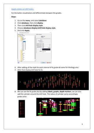
  • 3. 3 INTRODUCTION: Mine planning: Strength of a building depends on its strength of its foundation. Same is true for mining as well. As the foundation of all mining activity – a mine plan – most accurately reflects the real- time reality of the geological structure in the ground, the process capabilities and the economic unpredictability of demand and commodity markets; which results in a productive, predictable and profitable system within mining structure. To optimize mine profitability, planners and schedulers are under constant pressure to create mine plans that are as accurate as possible and optimize production at all stages, from mine to market. Geo-statistics: Geo-statistics is a branch of statistics focusing on spatial datasets. It is method of predicting probability distributions of ore grades for mining operations. It is intimately related to interpolation methods, but extends far beyond simple interpolation methods. This technique relies on statistical models that are based on random function theory to model the uncertainty associated with spatial estimation and simulation. Surpac: In this project we have used GEOVIA Surpac for studying and further planning of the mine using the data provided by the instructor. GEOVIA Surpac is the world’s most popular geology and mine planning software, supporting open pit and underground operations and exploration projects. Using Surpac, we can visualize an interpolation, lock it in 3-D and then we can bring in all the drilling, all the infrastructure, the development, the headings and know instantly whether we are on track. It also allows us integrate various processes to result a well-designed plan.
  • 4. 4 Overall Workflow Collect field data Make a Blank Database in Surpac Feed the field data in that blank database Display drillholes Sectioning Ore Modelling Compositing Grade Analysis using Histograms Variogram analysis and modelling Block Modelling and reserve estimation Ultimate Pit, Ramp Design and bench Design
  • 5. 5 Creating a Surpac Geological Database: Terminologies: - Geological Database: Geological database is the systematic collection of Drill Hole data. And drill hole data is starting of all the mine project. On the basis of this feasibility study and reserve estimation is done. A geological database consists of a number of tables, each of which contains different types of data. Each table contains a number of fields. Each table also has many records, with each record containing the data fields. Surpac use rational database model. For this project we use three mandatory table and three optional table for the geological database: Mandatory Tables: Collar, Survey, Translation Table (Surpac’s default) Optional Tables: Assay, Geology, Style table (surpac’s default) Collar Table: The information stored in the collar table describes the location of the drill hole collar, the maximum depth of the hole, and whether a linear or curved hole trace will be calculated when retrieving the hole. mandatory fields for collar table: hole_id, y, x, z, max_depth, hole_path Survey Table: The survey table stores the drill hole survey information used to calculate the drill hole trace coordinates. Mandatory fields for survey table: hole_id, depth, dip, azimuth Assay Table: Assay table is an Interval optional table (depth from to depth to) and assay table store information about the concentration of different components in an interval. Mandatory fields for Assay table: hole_id, depth_from, depth_to Optional fields that we have for assay table: percentages of fe, sio2, Al2O3, loi, p in an interval. Geology Table: It is also an Interval optional table. And it stores information about different geology in an interval. And the different geology of the field store as a code (0-10) known as lithocode(lcode). Mandatory fields for the geology table: hole_id, depth_from, depth_to, lcode Steps: Profile of surpac interface set as geological_database 1. Choose Database > Open/New. 2. Enter the name of database, and click Apply 3. Create definition for new database wizard open and click Apply 4. Choose database type as Access and click Apply
  • 6. 6 5. Mandatory table (collar, survey and translation table) already created after the above step. 6. Choose optional table i.e. Assay and Geology add these and define optional as interval 7. After that define all fields for all tables window appear and fill the assay table fields and geological table fields and add variable according to data we have. And click Apply
  • 7. 7 The database is created. The database name appears on the status line to indicate that you are connected to it. Two files have been created: 1. dream_database.mbd The Microsoft Access database which contains the data. 2. dream_ database.ddb The file that Surpac requires to connect to the database. Importing Drill Hole Data: For the importing of drill hole data in a database we have created first we have to connect database. Steps: 1. First, go to Database>import data. 2. Write format file name. Format file name is the name of the header. 3. Click Apply. Dream_database.dsc will created. . dsc is the file extension for a description file. 4. Click Apply. 5. Select the text file for each table. Select load type as insert and update. Click Apply. 6. Extra file also generates during this process with .rej file means rejected file. And all the error generated throughout process were encountered in these files.
  • 8. 8 7. Now all the tables imported and a report file also generated. 8. Now, we can view the imported tables by go to Edit>View tables>Select table name. 9. If we have to edit table then go to Edit>Edit tables>Select table name. 10. We can insert the new data by doing Edit>Insert records>Select table name. 11. And if we want to delete data then Edit>delete>select table name. Display Drill holes: Steps: 1. Firstly, we have to connect the database after that click Display Drillhole. 2. Then define query constraints form will be displayed. 3. Fill the necessary information and click Apply. 4. Then drill holes will be displayed in plan view.
  • 9. 9 Apply styles on dill holes: For the batter visualization and differentiate between the grades. Steps: 1. Go on the menu, and select database. 2. Click database, then click display. 3. Then click drill hole display style. 4. Choose database>display>drill hole display style. 5. And click Apply. 6. After adding all the style for each interval of fe grade do same for lithology also. 7. After that display drill hole for fe. 8. We can see the fe grade also by adding labels, graphs, depth markers. we can also add the cylinder around the drill hole. The radius of cylinder varies accordingly grade value.
  • 10. 10 Compositing: Terminology: Compositing: Compositing is a technique by which assay data are combined to form weighted average or composite grades representative of intervals longer than their own. After core is extracted and logged by the geologist and representative samples are sent out for assaying. Upon receipt, the assays are added to the other geological information such as length, depth, lithology etc. The se individual assay values may represent core lengths of a few inches up to many feet. Steps: 1. Choose Database > Composite > Downhole. 2. Enter the accordingly, and click Apply. Here we took compositing length of 5m. 3. In the report panel we can see the total number of samples, mean, number of boreholes that are processed etc. 4. This string file is generated.
  • 11. 11 5. White string shows the values having sample length greater than or equal to 3.75m. and the Blue string shows the values having sample length less than 3.75m. 6. We can see the statistics of sample data by right click on the string file and click Edit. Basic Statistics: Terminologies: Histogram: A histogram is a bar graph-like representation of data that buckets a range of outcomes into columns along the x-axis. The y-axis represents the number count or percentage of occurrences in the data for each column and can be used to visualize data distributions. Outlier: An outlier is an observation that lies an abnormal distance from other values in a random sample from a population. In a sense, this definition leaves it up to the analyst (or a consensus process) to decide what will be considered abnormal. Steps: 1. For opening the basic statistics window in surpac click Database>Analysis>Basic statistics window.
  • 12. 12 2. Click file>Load data from string file. select the string file. and Click Apply. And histogram will appear with cumulative frequency curve. 3. We can only see the histogram by click display>histogram. And save histogram by clicking save icon. 4. Normal distribution curve of data made by clicking on Display>normal distribution curve.
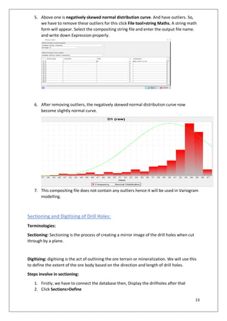
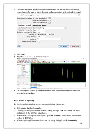
  • 13. 13 5. Above one is negatively skewed normal distribution curve. And have outliers. So, we have to remove these outliers for this click File tool>string Maths. A string math form will appear. Select the compositing string file and enter the output file name. and write down Expression properly. 6. After removing outliers, the negatively skewed normal distribution curve now become slightly normal curve. 7. This compositing file does not contain any outliers hence it will be used in Variogram modelling. Sectioning and Digitising of Drill Holes: Terminologies: Sectioning: Sectioning is the process of creating a mirror image of the drill holes when cut through by a plane. Digitizing: digitising is the act of outlining the ore terrain or mineralization. We will use this to define the extent of the ore body based on the direction and length of drill holes. Steps involve in sectioning: 1. Firstly, we have to connect the database then, Display the drillholes after that 2. Click Sections>Define
  • 14. 14 3. Define slicing planes width window will open define the section definition method, enter distance forward of plane, distance backward of plane and section by interval. 4. Click Apply 5. After that one section of drill hole appear. 6. For viewing next section go to sections>Next. And we can see the previous section also sections>Previous. Steps involve in Digitizing: For digitizing already define section we have to follow these steps: 1. Click create>digitise>New point 2. Then digitise end points of ore zone by clicking the right click and choose the point and covers all the drill hole boundaries. 3. After one section digitization complete go to section>next and do same for the next section of drill holes. 4. After completing of all the sections save the string file by go to File>save>string.
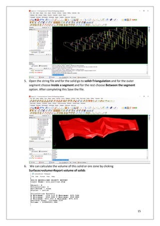
  • 15. 15 5. Open the string file and for the solid go to solid>Triangulation and for the outer segment choose Inside a segment and for the rest choose Between the segment option. After completing this Save the file. 6. We can calculate the volume of this solid or ore zone by clicking Surfaces>volume>Report volume of solids
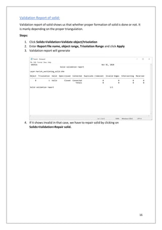
  • 16. 16 Validation Report of solid: Validation report of solid shows us that whether proper formation of solid is done or not. It is manly depending on the proper triangulation. Steps: 1. Click Solids>Validation>Validate object/trisolation 2. Enter Report file name, object range, Trisolation Range and click Apply 3. Validation report will generate 4. If it shows invalid in that case, we have to repair solid by clicking on Solids>Validation>Repair solid.
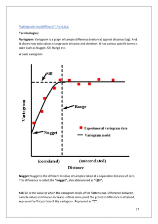
  • 17. 17 Variogram modelling of the data: Terminologies: Variogram: Variogram is a graph of sample difference (variance) against distance (lag). And it shows how data values change over distance and direction. It has various specific terms is used such as Nugget, Sill, Range etc. A basic variogram: Nugget: Nugget is the different in value of samples taken at a separation distance of zero. This difference is called the “nugget”, also abbreviated as “c(0)”. Sill: Sill is the value at which the variogram levels off or flattens out. Difference between sample values continuous increase until at some point the greatest difference is attained, represent by flat portion of the variogram. Represent as “C”.
  • 18. 18 Total sill: Total sill is the nugget to sill ratio. (nugget / (nugget + sill) Range: Range is the maximum distance at which the sill attained. Sometime represented as “A”. After the range there is no relationship between data. Isotropy Data: Isotropy means the values measured in different direction are same. Anisotropy Data: Anisotropy means having the difference value in different direction. Omnidirectional variogram: In omnidirectional variogram, sample pairs are selected based only on their separation distance. Directional variogram: In this, sample pairs are selected based on a particular direction or orientation. Variogram analysis consists of the experimental variogram calculated from the data and the variogram model fitted to the data. Steps: 1. For opening of variogram window click Block model>Geostatistics>Variogram modelling. 2. For the experiment variogram first we should have Compositing String file for fe without any outlier. So, we have to remove all the outlier before the variogram analysis. 3. Now for the experiment variogram from data click File>New>String file variogram. 4. After that variogram calculation window will appear. Fill all the required options accordingly. We choose firstly Lag distance 10, maximum distance ( it is around the half of the distance between the outer segment of the ore or half of total extended ore) is around 625 m. In this we also get advance option for variogram calculation in which we can add Geographical constrain and properties of Lag slider. 5. After filling all the details click Apply.
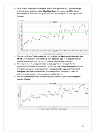
  • 19. 19 6. After that an experimental variogram appear with lag distance 10. We can change the lag distance by click on right side of Lag slider. We changed at 20 for better representation. If we took the lag distance low then no of pairs at each lag distance increase. 7. There are different Variogram Model such as Spherical, Exponential, Gaussian, Hole Effect. So, try each one for best fitting. Here Spherical type of variogram used for modelling because it gave the best fit curve on experimental variogram. 8. Now, we have to fit variogram model on this experiment variogram for the calculation of different attributes of it. So, for that click Variogram>model or we can change the variogram model by click on variogram model type. With the help of variogram structure try to fit model on the experiment variogram. At least 3-4 points of model should be lies on experimental variogram. 9. And, we can see the number of pair for each lag distance by click on display/hide number of pairs.
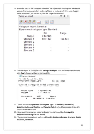
  • 20. 20 10. When we best fit the variogram model on the experimental variogram we see the values of various parameters on the right side of variogram. In this case, Nugget value is around 2, sill around 50, and the range is around 130. 11. For the report of variogram click Variogram>Report. And enter the file name and click Apply. Report will generate in not file. 12. There is various Experimental variogram type i.e. standard, Normalised, Logarithmic, General Relative and Pairwise Relative. So, Choose accordingly. We choose standard for this. 13. Now save the variogram model and experimental model by click save the experimental variogram and model. 14. There are various options such as add model, delete model, add structure, Delete structure, validation.
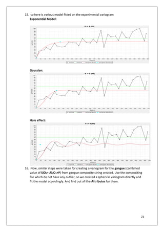
  • 21. 21 15. so here is various model fitted on the experimental variogram Exponential Model: Gaussian: Hole effect: 16. Now, similar steps were taken for creating a variogram for the gangue (combined value of SiO2+ Al2O3+P) from gangue composite string created. Use the compositing file which do not have any outlier, so we created a spherical variogram directly and fit the model accordingly. And find out all the Attributes for them.
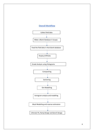
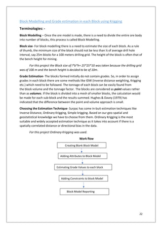
  • 22. 22 Block Modelling and Grade estimation in each Block using Krigging Terminologies: - Block Modelling – Once the ore model is made, there is a need to divide the entire ore body into number of blocks, this process is called Block Modelling. Block size- For block modelling there is a need to estimate the size of each block. As a rule of thumb, the minimum size of the block should not be less than ¼ of average drill hole interval, say 25m blocks for a 100 meters drilling grid. The height of the block is often that of the bench height for mining. For this project the Block size of l*b*h= 25*25*10 was taken because the drilling grid was of 100 m and the bench height is decided to be of 10m. Grade Estimation- The blocks formed initially do not contain grades. So, in order to assign grades in each block there are some methods like IDW (Inverse distance weighting, Krigging etc.) which need to be followed. The tonnage of each block can be easily found from the block volume and the tonnage factor. The blocks are considered as point values rather than as volumes. If the block is divided into a mesh of smaller blocks, the calculation would be made for each sub-block and the results summed. Hughes & Davey (1979) has indicated that the difference between the point and volume approach is small. Choosing the Estimation Technique- Surpac has some in-buit estimation techniques like Inverse Distance, Ordinary Krigging, Simple krigging. Based on our geo-spatial and geostatistical knowledge we have to choose from them. Ordinary Krigging is the most suitable and widely accepted estimation technique as it takes into account if there is a spatially correlated distance or directional bias in the data. For this project Ordinary Krigging was used. Work flow Creating Blank Block Model Adding Attributes to Block Model Estimating Grade Values to each block Adding Constraints to block Model Block Model Reporting
  • 23. 23 Steps: Creating Blank block model. 1. Open ore model.dtm 2. Click Display > 3D Grids and note down the approx. extents of the ore body. For this project Northing was found to be in the range [-900 to 500], Easting in the range [-300 to 500], Elevation in the range [600 to 900]. (all values in meter) 3. Click Block Model > Block Model > New/Open. 4. A ‘Select Model’ dialogue box appears. Enter Model Name, say block_model_1. Click Apply. Then again, a dialogue box appears, Click Apply. 5. ‘Creating new block model definition’ Window appears. Enter the Coordinate extents of X, Y, Z which has been found in Step-2. Coordinate Extents can also be input from the Sectioning string file. Enter block size which has been decided earlier. In Sub blocking choose Standard and Minimum block size of 6.25,6.25,2.5. Click Apply.
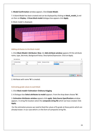
  • 24. 24 6. Model Confirmation window appears. Click Create Model. 7. A blank Model has been created and can be displayed by clicking on block_model_1 and on then on Display. A Draw block model dialogue box appears click Apply. 8. Block model is displayed. Adding attributes to the block model 1. Click Block Model> Attributes> New. An Add attribute window appears.Fill the attribute name, type, decimals, Background Value, Description/Expression. Click on Apply. 2. Attribute with name ‘fe’ is created. Estimating grade values to each block 1. Click Block model> Estimation> Ordinary Krigging 2. A Dialogue box Select attributes to model appears. From the drop down choose ‘fe’. 3. Estimation Attributes window appears click apply. Data Source Specifications window appears. In string file location select the composite string file which we have created. Click Apply. For the estimation process we need to feed the values of fe grade at those points which are already known. In our case which is in the form of composite string file.
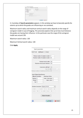
  • 25. 25 4. A window of Search parameters appears. In this window we have to basically specify the extents up to which the grades are influencing or are corelated. Maximum search radius and maximum vertical search radius depends on the range of variogram model in case of krigging. This precisely explains that up-to how much distance the grades are having their influence. In this particular case the range of the variogram model was around 130. Maximum search radius- 130 Maximum Vertical search radius- 130 Click Apply. .
  • 26. 26 5. Krigging Parameters window opens. In the variogram file name Insert the variogram model created. In number of discretisation point fill X=3, Y=3, Z=3. This basically denotes the direction in which the grades are having their influence. If a greater number of points are selected it will take more time to estimate but will give better estimation. Write the report file name and format. Click Apply. 6. The grades have been applied to each block. To see the grade of a particular block. Click Block Model> Attributes> View attributes of one block. Then click on the block of which you wish to see the grade value. Adding Constraints to Block Model: Constraints are added to constrain our block model to a particular value, blocks or DTM. 1. Click on Block Model> Constraints> New Constraints file. 2. In the add constraints window Select the constraint type then select the file under which we have to constrain the block model. Click Add and then Apply Block Model Reporting Used to report the whole block model. 1. Choose Block Model> Report. 2. Enter the Output report file name and click Apply. 3. Block Model report window opens. In report attributes select the attributes which we have to report. In this case fe was chosen. If we want our report to contain weight then specific gravity should be provided in the density arrangement. Groupby attributes is used to subgroups the different attributes. In this case the fe attribute was further divided into 0- 47.5, 47.5-57.5, 57.5-999 and for Z value 600-700,700-800,800-900. Click Apply.
  • 27. 27 4. Enter constraints window appears. Select 3DM as constraint type and Ore_model.dtm as the constraint file. This will constraint the report which is going to be generated within that ore model solid. Click Apply. 5. A notepad file containing report appears. This file shows the different values of tonnage, volume for different grades of ore.
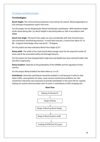
  • 28. 28 Pit design and Ramp design: Terminologies- Bench Height- The vertical distance between crest and toe of a bench. Mainly dependent on size and type of equipment used in the mine. For this project we are designing for Shovel and Dumper combination. With maximum height of the shovel being 10m. So, Bench Height is also being taken as 10m in accordance with MMR. Bench Face Angle- The bench face angle can vary considerably with rock characteristics, face orientation and blasting practices. In most hard rock pits, it varies from about 55◦ to 80◦. A typical initial design value may be 65 – 70 degree. For this project we have selected a Bench Face Angle of 55. Ramp width- The width of the road should allow enough room for the required number of lanes and all the associated safety and drainage features. For this project we have designed both single lane and double lane haul road with width 14m and 28 m respectively. Ramp Gradient- Depends on the gradeability of the HEMMs and the regulation of that country. For this project Ramp Gradient has been taken as 1 in 16. Switchbacks- Generally switchbacks should be avoided in a pit because it tends to slow down traffic, cause greater tire wear, cause various maintenance problems etc. But sometimes it becomes very necessary to provide switchbacks in the cases like for a gently sloping ore contact which provides room to work in switchbacks at little stripping cost. Work Flow Making of Ultimate Pit Design of Ramp Design of Bench by Bench Height Design of Bench by berm width Creating of DTM from Pit Layout
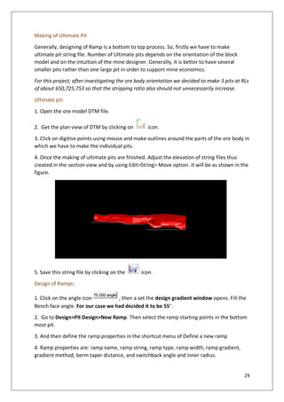
  • 29. 29 Making of Ultimate Pit Generally, designing of Ramp is a bottom to top process. So, firstly we have to make ultimate pit string file. Number of Ultimate pits depends on the orientation of the block model and on the intuition of the mine designer. Generally, it is better to have several smaller pits rather than one large pit in order to support mine economics. For this project, after investigating the ore body orientation we decided to make 3 pits at RLs of about 650,725,753 so that the stripping ratio also should not unnecessarily increase. Ultimate pit: 1. Open the ore model DTM file. 2. Get the plan view of DTM by clicking on icon. 3. Click on digitise points using mouse and make outlines around the parts of the ore body in which we have to make the individual pits. 4. Once the making of ultimate pits are finished. Adjust the elevation of string files thus created in the section view and by using Edit>String> Move option. It will be as shown in the figure. 5. Save this string file by clicking on the icon. Design of Ramps: 1. Click on the angle icon , then a set the design gradient window opens. Fill the Bench face angle. For our case we had decided it to be 55. 2. Go to Design>Pit Design>New Ramp. Then select the ramp starting points in the bottom most pit. 3. And then define the ramp properties in the shortcut menu of Define a new ramp 4. Ramp properties are: ramp name, ramp string, ramp type, ramp width, ramp gradient, gradient method, berm taper distance, and switchback angle and inner radius.
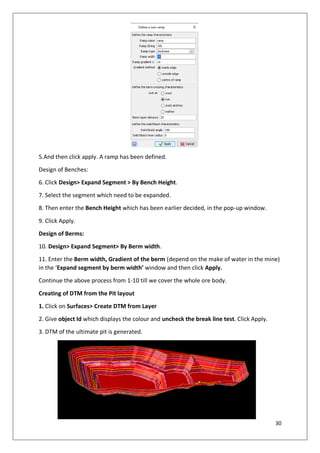
  • 30. 30 5.And then click apply. A ramp has been defined. Design of Benches: 6. Click Design> Expand Segment > By Bench Height. 7. Select the segment which need to be expanded. 8. Then enter the Bench Height which has been earlier decided, in the pop-up window. 9. Click Apply. Design of Berms: 10. Design> Expand Segment> By Berm width. 11. Enter the Berm width, Gradient of the berm (depend on the make of water in the mine) in the ‘Expand segment by berm width’ window and then click Apply. Continue the above process from 1-10 till we cover the whole ore body. Creating of DTM from the Pit layout 1. Click on Surfaces> Create DTM from Layer 2. Give object Id which displays the colour and uncheck the break line test. Click Apply. 3. DTM of the ultimate pit is generated.
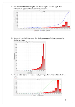
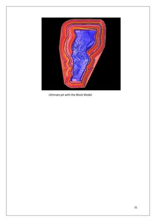
  • 31. 31 Ultimate pit with the Block Model
  • 32. 32 Results and Conclusion: Extents of Ore Body Minimum Maximum X -224.113 425.544 Y -850 450 Z 425.544 425.544 Volume, mass and average grade The average grade of Fe as estimated by Ordinary Krigging method was 60.422 and the total tonnage of Ore estimated was 2.35*108 tonnes. (Sp. Gravity of 5.5 was used).
  • 33. 33 Pit Design: Assumptions: 1. Shovel- Dumper combination to be deployed. 2. Electrical Rope Shovel with maximum digging height= 10,300 mm= 10.3 m 3. Komatsu 100 tonne dumpers with width= 4663.2 mm = 4.6 m Based on these assumptions and keeping the Metal Mines Regulations in account. The following pit design parameters had been selected Bench Height=10m Ramp Width= 14 m Ramp Gradient= 1:16 Berm Width= 5m. Final View of the pit.
close