Applying Python Programming to Solve Mechanical Engineering Problems

Using Python Programming to solve PDV work problems

In cases of closed systems which are also called as systems where the identity of mass does not change, the system interacts with its surroundings either in terms of heat or work. In this article, we will be dealing with the non-dissipative work interaction which is also known as the PDV or displacement work. We will be using Python programming to solve these problems.

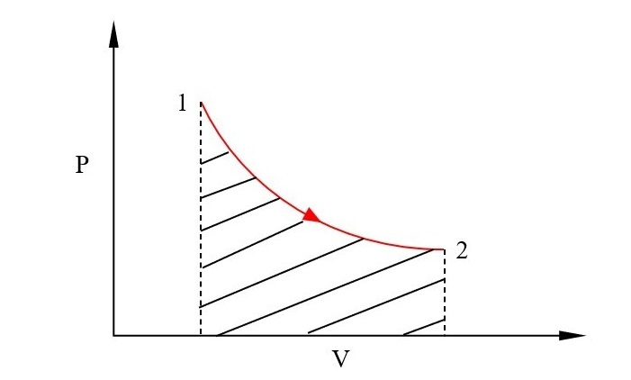
But before we start, one should know the fundamental meaning of displacement work. The displacement work is evaluated as the integral of the path the system has taken between end states in the pressure-volume plot given below.

For this work to be evaluated the path must be completely specified which is only possible when the process is quasi-static. In the plot, the area under the curve (1-2) is nothing but the work done. Mathematically, it is written as Follows ?

Following is a pressure-volume plot for a typical process 1-2 ?

Implementation

Now, as we have already mentioned that, to evaluate PDV work the path has to be completely specified. Therefore, to implement it in Python a relation between pressure and volume should be known. Also, the end information about pressure or volume should be known in advance. The methodology to solve the problem will be as follows ?

• A function has to be developed to specify the relation between p and v.
• Input parameters are to be supplied.
• The constant on the right-hand side has to be evaluated based on input data.
• The number of data points to be created between endpoints (n) has to be provided.
• The spacing between data points (h) is evaluated and the array of volume is created.
• Numerical integration will be used to solve the problem.
• Finally, to plot the process, Pylab (a python module to plot) along with NumPy will be used.

Mathematical Formula

For a function f(x) between endpoints a and b, the numerical integration can be simply performed using the Trapezoidal rule as ?

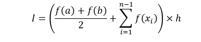
Here, the index i starts from 0 and ends at n. So, x₀=a and x_n=b.

The process where, pv=constant

To understand the process let us first consider a problem in which the pressure-volume relation is given by, pv=c. We will write the code in pieces and explain after each piece what it is doing.

# importing modules from pylab import * from numpy import * 

Here in this portion of code the modules ?pylab' and ?numpy' are called for the data plotting and array creation, respectively.

# defining function for pv relation def p(v,C): return C/v 

Here, a function is defined that accepts two arguments viz. volume and the constant C (the RHS of pv=c). This function can be modified based on the thermodynamic process given and the initial conditions.

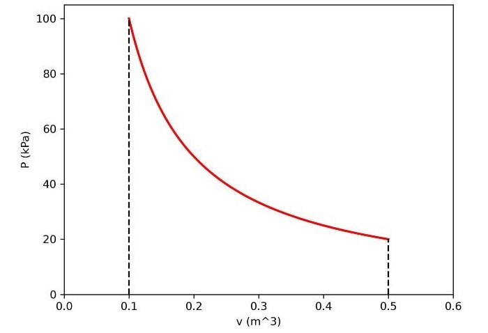
# input data #--------------- # Initial and final volume (in m^3) v1 = 0.1 v2 = 0.5 # initial pressure (in kPa) p1 = 100 

Then the input data is supplied to the program. Here in this problem, we have assumed that the volume at the end points is known along with the initial pressure.

# Evaluating C C=p1*v1 # Number of data points between end points n=5000 # Spacing between data points h=(v2-v1)/n # creating array of volume v=linspace(v1, v2,n) 

The based-on input data constant C is evaluated. The number of data points between end points has to be supplied (as we have used Trapezoidal rule, so more the number of data points more will be the accuracy). The spacing between the data points is evaluated and an array of volume is created.

 # Numerical Integration f_a=p(v1,C) f_b=p(v2,C) Sum=0 for i in range(1,n-1): Sum=Sum+p(v[i],C) I=h*((f_a+f_b)/2+Sum) # work done Work = I print(f'Work = {round(Work,3)} kJ') 

In this step, numerical integration is performed using the formula as mentioned in the previous section. Then the result of integration is transferred to the variable ?Work' (for the sake of simplicity) and the result is printed. For plotting the process, the following piece of code can be used which uses the print() function to perform the task of plotting.

 # Data plotting figure(1,dpi=300) plot(v,p(v,C),'r',linewidth=2) xlabel('v (m^3)') ylabel('P (kPa)') ylim(0,p1+5) xlim(0,v2+0.1) plot([v1,v1],[0,p1],'--k') p2=C/v2 plot([v2,v2],[0,p2],'--k') savefig('work.jpg') 

The program output will be as follows ?

Work = 16.091 kJ 

The process where, pv^n=c

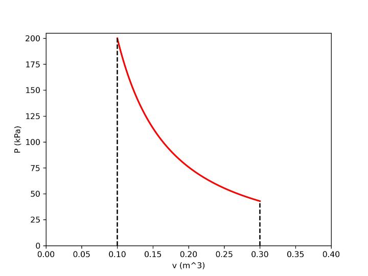
Let's say we have evaluated the work done in the process pv^n, where n is known to us. This time we will assume that pressure at the end points is known, and the initial volume is known. The only change this time will be in the function we are creating for the relation between p-v and the input parameters.

Here we are assuming that v1, v2, and p1 as 0.1 m3, 0.3 m3, and 200 kPa, respectively. Also, assume n=1.4. The Python program to compute the work done in the process along with the data plotting is as follows ?

 # importing modules from pylab import * from numpy import * # defining function for pv relation def p(v,C,N): return C/v**N # input data #--------------- # Initial and final volume (in m^3) v1 = 0.1 v2 = 0.3 # initial pressure (in kPa) p1 = 200 # Exponent n N=1.4 # Evaluating C C=p1*v1**N # Number of data points between end points n=5000 # Spacing between data points h=(v2-v1)/n # creating array of volume v=linspace(v1, v2,n) # Numerical Integration f_a=p(v1,C,N) f_b=p(v2,C,N) Sum=0 for i in range(1,n-1): Sum=Sum+p(v[i],C,N) I=h*((f_a+f_b)/2+Sum) # work done Work2 = I print(f'Work = {round(Work2,3)} kJ') # Data plotting figure(1,dpi=300) plot(v,p(v,C,N),'r',linewidth=2) xlabel('v (m^3)') ylabel('P (kPa)') ylim(0,p1+5) xlim(0,v2+0.1) plot([v1,v1],[0,p1],'--k') p2=C/v2**N plot([v2,v2],[0,p2],'--k') savefig('work2.jpg') 

The program output will be as follows ?

Work = 17.777 kJ 

Now in this article, you have observed how one can evaluate closed systems work with the help of Python. The procedure mentioned above can be easily applied to different processes or different initial conditions with slight changes in the function, arrays, and input parameters.