ML | Data Preprocessing in Python

Data preprocessing is a important step in the data science transforming raw data into a clean structured format for analysis. It involves tasks like handling missing values, normalizing data and encoding variables. Mastering preprocessing in Python ensures reliable insights for accurate predictions and effective decision-making. Pre-processing refers to the transformations applied to data before feeding it to the algorithm.

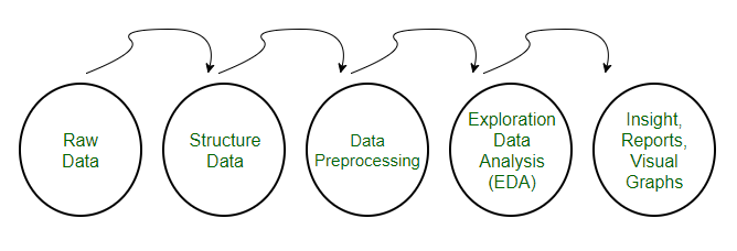
Data Preprocessing

Steps in Data Preprocessing

Step 1: Import the necessary libraries

# importing librariesimportpandasaspdimportscipyimportnumpyasnpfromsklearn.preprocessingimportMinMaxScalerimportseabornassnsimportmatplotlib.pyplotasplt

Step 2: Load the dataset

You can download dataset from here.

# Load the datasetdf=pd.read_csv('Geeksforgeeks/Data/diabetes.csv')print(df.head())

Output:

 Pregnancies Glucose BloodPressure SkinThickness Insulin BMI 0 6 148 72 35 0 33.6 \ 1 1 85 66 29 0 26.6 2 8 183 64 0 0 23.3 3 1 89 66 23 94 28.1 4 0 137 40 35 168 43.1 DiabetesPedigreeFunction Age Outcome 0 0.627 50 1 1 0.351 31 0 2 0.672 32 1 3 0.167 21 0 4 2.288 33 1

1. Check the data info

df.info()

Output:

<class 'pandas.core.frame.DataFrame'> RangeIndex: 768 entries, 0 to 767 Data columns (total 9 columns): # Column Non-Null Count Dtype --- ------ -------------- ----- 0 Pregnancies 768 non-null int64 1 Glucose 768 non-null int64 2 BloodPressure 768 non-null int64 3 SkinThickness 768 non-null int64 4 Insulin 768 non-null int64 5 BMI 768 non-null float64 6 DiabetesPedigreeFunction 768 non-null float64 7 Age 768 non-null int64 8 Outcome 768 non-null int64 dtypes: float64(2), int64(7) memory usage: 54.1 KB

As we can see from the above info that the our dataset has 9 columns and each columns has 768 values. There is no Null values in the dataset.

We can also check the null values using df.isnull()

df.isnull().sum()

Output:

Pregnancies 0 Glucose 0 BloodPressure 0 SkinThickness 0 Insulin 0 BMI 0 DiabetesPedigreeFunction 0 Age 0 Outcome 0 dtype: int64

Step 2: Statistical Analysis

In statistical analysis we use df.describe() which will give a descriptive overview of the dataset.

df.describe()

Output:

Data summary

The above table shows the count, mean, standard deviation, min, 25%, 50%, 75% and max values for each column. When we carefully observe the table we will find that Insulin, Pregnancies, BMI, BloodPressure columns has outliers. 

Let’s plot the boxplot for each column for easy understanding.

Step 3: Check the outliers

# Box Plotsfig,axs=plt.subplots(9,1,dpi=95,figsize=(7,17))i=0forcolindf.columns:axs[i].boxplot(df[col],vert=False)axs[i].set_ylabel(col)i+=1plt.show()

Output:

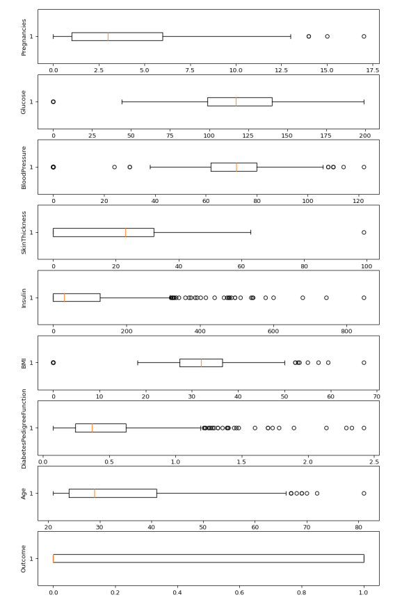
Boxplots

from the above boxplot we can clearly see that every column has some amounts of outliers. 

Step 4: Drop the outliers

# Identify the quartilesq1,q3=np.percentile(df['Insulin'],[25,75])# Calculate the interquartile rangeiqr=q3-q1# Calculate the lower and upper boundslower_bound=q1-(1.5*iqr)upper_bound=q3+(1.5*iqr)# Drop the outliersclean_data=df[(df['Insulin']>=lower_bound)&(df['Insulin']<=upper_bound)]# Identify the quartilesq1,q3=np.percentile(clean_data['Pregnancies'],[25,75])# Calculate the interquartile rangeiqr=q3-q1# Calculate the lower and upper boundslower_bound=q1-(1.5*iqr)upper_bound=q3+(1.5*iqr)# Drop the outliersclean_data=clean_data[(clean_data['Pregnancies']>=lower_bound)&(clean_data['Pregnancies']<=upper_bound)]# Identify the quartilesq1,q3=np.percentile(clean_data['Age'],[25,75])# Calculate the interquartile rangeiqr=q3-q1# Calculate the lower and upper boundslower_bound=q1-(1.5*iqr)upper_bound=q3+(1.5*iqr)# Drop the outliersclean_data=clean_data[(clean_data['Age']>=lower_bound)&(clean_data['Age']<=upper_bound)]# Identify the quartilesq1,q3=np.percentile(clean_data['Glucose'],[25,75])# Calculate the interquartile rangeiqr=q3-q1# Calculate the lower and upper boundslower_bound=q1-(1.5*iqr)upper_bound=q3+(1.5*iqr)# Drop the outliersclean_data=clean_data[(clean_data['Glucose']>=lower_bound)&(clean_data['Glucose']<=upper_bound)]# Identify the quartilesq1,q3=np.percentile(clean_data['BloodPressure'],[25,75])# Calculate the interquartile rangeiqr=q3-q1# Calculate the lower and upper boundslower_bound=q1-(0.75*iqr)upper_bound=q3+(0.75*iqr)# Drop the outliersclean_data=clean_data[(clean_data['BloodPressure']>=lower_bound)&(clean_data['BloodPressure']<=upper_bound)]# Identify the quartilesq1,q3=np.percentile(clean_data['BMI'],[25,75])# Calculate the interquartile rangeiqr=q3-q1# Calculate the lower and upper boundslower_bound=q1-(1.5*iqr)upper_bound=q3+(1.5*iqr)# Drop the outliersclean_data=clean_data[(clean_data['BMI']>=lower_bound)&(clean_data['BMI']<=upper_bound)]# Identify the quartilesq1,q3=np.percentile(clean_data['DiabetesPedigreeFunction'],[25,75])# Calculate the interquartile rangeiqr=q3-q1# Calculate the lower and upper boundslower_bound=q1-(1.5*iqr)upper_bound=q3+(1.5*iqr)# Drop the outliersclean_data=clean_data[(clean_data['DiabetesPedigreeFunction']>=lower_bound)&(clean_data['DiabetesPedigreeFunction']<=upper_bound)]

Step 5: Correlation

#correlationcorr=df.corr()plt.figure(dpi=130)sns.heatmap(df.corr(),annot=True,fmt='.2f')plt.show()

Output:

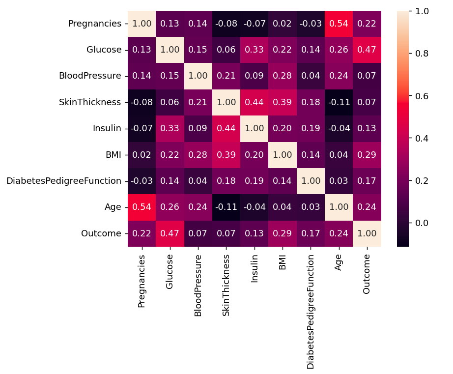
Correlation

We can also compare by single columns in descending order

corr['Outcome'].sort_values(ascending=False)

Output:

Outcome 1.000000 Glucose 0.466581 BMI 0.292695 Age 0.238356 Pregnancies 0.221898 DiabetesPedigreeFunction 0.173844 Insulin 0.130548 SkinThickness 0.074752 BloodPressure 0.0

Step 6: Check Outcomes Proportionality

plt.pie(df.Outcome.value_counts(),labels=['Diabetes','Not Diabetes'],autopct='%.f',shadow=True)plt.title('Outcome Proportionality')plt.show()

Output:

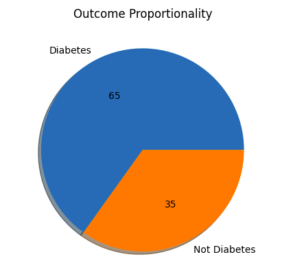
Outcome Proportionality

Step 7: Separate independent features and Target Variables

# separate array into input and output componentsX=df.drop(columns=['Outcome'])Y=df.Outcome

Step 7: Normalization or Standardization

Normalization

• Normalization works well when the features have different scales and the algorithm being used is sensitive to the scale of the features, such as k-nearest neighbors or neural networks.
• Rescale your data using scikit-learn using the MinMaxScaler.
• MinMaxScaler scales the data so that each feature is in the range [0, 1]. 

# initialising the MinMaxScalerscaler=MinMaxScaler(feature_range=(0,1))# learning the statistical parameters for each of the data and transformingrescaledX=scaler.fit_transform(X)rescaledX[:5]

Output:

array([[0.353, 0.744, 0.59 , 0.354, 0. , 0.501, 0.234, 0.483], [0.059, 0.427, 0.541, 0.293, 0. , 0.396, 0.117, 0.167], [0.471, 0.92 , 0.525, 0. , 0. , 0.347, 0.254, 0.183], [0.059, 0.447, 0.541, 0.232, 0.111, 0.419, 0.038, 0. ], [0. , 0.688, 0.328, 0.354, 0.199, 0.642, 0.944, 0.2 ]])

Standardization

• Standardization is a useful technique to transform attributes with a Gaussian distribution and differing means and standard deviations to a standard Gaussian distribution with a mean of 0 and a standard deviation of 1.
• We can standardize data using scikit-learn with the StandardScaler class.
• It works well when the features have a normal distribution or when the algorithm being used is not sensitive to the scale of the features

fromsklearn.preprocessingimportStandardScalerscaler=StandardScaler().fit(X)rescaledX=scaler.transform(X)rescaledX[:5]

Output:

array([[ 0.64 , 0.848, 0.15 , 0.907, -0.693, 0.204, 0.468, 1.426], [-0.845, -1.123, -0.161, 0.531, -0.693, -0.684, -0.365, -0.191], [ 1.234, 1.944, -0.264, -1.288, -0.693, -1.103, 0.604, -0.106], [-0.845, -0.998, -0.161, 0.155, 0.123, -0.494, -0.921, -1.042], [-1.142, 0.504, -1.505, 0.907, 0.766, 1.41 , 5.485]

In conclusion data preprocessing is an important step to make raw data clean for analysis. Using Python we can handle missing values, organize data and prepare it for accurate results. This ensures our model is reliable and helps us uncover valuable insights from data.

GeeksforGeeks

Improve

Article Tags :

• AI-ML-DS
• Machine Learning
• AI-ML-DS With Python

Practice Tags :

• Machine Learning