

Abstract
With the onset of COVID-19 restrictions and the slow relaxing of many restrictions, it is imperative that we understand what this means for the performance of the transport network. In going from almost no commuting, except for essential workers, to a slow increase in travel activity with working from home (WFH) continuing to be both popular and preferred, this paper draws on two surveys, one in late March at the height of restrictions and one in late May as restrictions are starting to be partially relaxed, to develop models for WFH and weekly one-way commuting travel by car and public transport. We compare the findings as one way to inform us of the extent to which a sample of Australian residents have responded through changes in WFH and commuting. While it is early days to claim any sense of a new stable pattern of commuting activity, this paper sets the context for ongoing monitoring of adjustments in travel activity and WFH, which can inform changes required in the revision of strategic metropolitan transport models as well as more general perspectives on future transport and land use policy and planning.
Keywords: Coronavirus, COVID-19, Travel activity, Working from home (WFH), Ordered logit WFH model, Frequency of modal commuting, Poisson regression, Household surveys, Australian evidence
Highlights
- •
Two wave study examining work from home (WFH) and commute behaviour through COVID-19 pandemic.
- •
New models for WFH and impact on commuting activity.
- •
Evidence of changes WFH and commuting from immediately after restrictions to their initial easing
- •
Small decreases in WFH and increases in car-based commuting starting to occur.
- •
WFH has been a positive experience and many would to WFH more than before COVID-19, if they have an appropriate space.
- •
Policy makers should encourage employer support for working from home and help identify and reduce barriers to doing so.
1. Introduction
The COVID-19 pandemic was brought to the centre of Australian consciousness at the beginning of March 2020, with the first death in Australia occurring on the 1st of March. On the 13th of March, Australia formed the National Cabinet, designed to coordinate government response at all levels to the rising infection rate within the country. As a result, a series of regulations were brought to bear, many of which curtailed movement and changed the nature of work and commuting in Australia. Research conducted early in the restriction process (first two weeks of April) revealed just how widespread those changes were (Beck and Hensher, 2020).
As a result of the suppression of travel and activities, Australia has been able to also supress the rate of COVID-19 infection. Fig. 1 shows the number of daily new cases of COVID-19, with the two waves of the survey carried out as part of the research reported below. These surveys asked respondents to reflect on travel and activities during the height of the initial spike in new cases, and in Wave 2 during a period of relatively low new infections, when discussion was turning towards a staged relaxation of restrictions.
Fig. 1.

Daily New Cases of COVID-19 in Australia.
Source:https://www.health.gov.au/news/health-alerts/novel-coronavirus-2019-ncov-health-alert
In early May, the Federal government announced a three-stage plan devised by National Cabinet to ease restrictions across the country, with each state and territory to decide when each stage will be implemented within their jurisdiction. For example, a key date in NSW was July 1st, wherein the number of people allowed inside indoor venues is now determined by the ‘one person per 4 square metre’ rule, with no upper limit. Cultural and sporting events at outdoor venues with a maximum capacity of 40,000 were allowed, but only up to 25% of their normal capacity. On compassionate grounds, restrictions on funerals were eased to allow the four-square metre rule to apply. Restrictions including 20 guests inside the home and 20 for outside gatherings remained the same.
As a note, Fig. 1 also reveals a climbing number of new cases towards the end of June, in part due to travellers returning home to Australia testing positive (returning travellers are tested and are required to quarantine in hotels for 14 days upon arrival, the cost of which is borne by the government),1 but more concerning a sharp rise in community transfer of COVID-19 in a number of suburbs in Melbourne.2 This emphasises the importance of not only the continual monitoring of COVID-19 infection rates, but also the regular assessment and modelling of travel and activity patterns of Australians during this period of instability.
Previous insight on working from home had been provided in Australian Bureau of Statistics Labour Force surveys (ABS, 2020a) and Personal Employed at Home surveys (ABS, 2020b), but little work has been done to link that with travel data. The current context offers an opportunity for a fresh examination of this issue. As such, the focus of this paper is identifying the relationship between the number of days working from home at the height of COVID-19 restrictions (late March 2020) and as restriction began to be relaxed in late May, and the amount of modal travel associated with commuting to and from the pre-COVID-19 work place. As might be expected, and as shown above, the amount of commuting activity outside of the home was initially severely curtailed either by employee choice, by employer command, or by government restrictions3 and slowly began to increase as restrictions were relaxed.
The objective of this paper is not to discuss working from home and related issues in great detail, which is the main focus of two other papers by Beck and Hensher, 2020, Beck and Hensher, 2020a; rather we attempt to set the context for ongoing monitoring of adjustments in travel activity and WFH, which can inform changes required in the revision of strategic metropolitan transport models as well as more general perspectives on future transport and land use policy and planning. However, detail on experiences with working from home will be provided for context within this paper.
This paper is structured as follows: section two provides an overview of the working from home literature, section three provides results on the level of working from home and the experiences therein for the collected data; section four outlines the modelling approach to estimate the influences on days worked from home and number of commuting trips made; section five discusses the results of the modelling; section six presents scenario analysis wherein working from home and commuting trips are simulated under different assumptions; section seven provides discussion of results and suggestions for future research to address the limitations of this study; and section eight provides the conclusion.
2. Literature review
Working from home has long been of interest to transport researchers, with the concept of telecommuting first being formed by Nilles (1973) who proposed the substitution of commuting for “telecommuting” (working at home made possibly by technological advances) in response to traffic, sprawl, and scarcity of non-renewable resources. In early work the focus was mainly on white collar workers in the information technology sector (Salomon and Salomon 1984), and many looked barriers which might exist to working from home such as lack of social interaction, inability to separate home from work, and feeling that there was a need to be seen in order to advance (Salomon, 1986; Hall, 1989). Nonetheless, the concept of working from home gained traction in the transport literature as a relatively fast and inexpensive way to overcome several problems associated with congestion and it was argued that the impact of telecommuting on traditional transport demand models needed to be considered (Mokhtarian, 1991).
Ben-Akiva et al. (1996) proposed a travel demand modelling framework for the information era. They outline a three stage approach to incrementally updating the forecasting process through understanding how lifestyle decisions impact on mobility choices and how both impact on daily activity patterns. While Ben-Akiva et al. (1996) include sampling of both employees and employers, Yen and Mahmassani (1997) include both from the same organisation. The role of social influence and social contact on telecommuting has also been explored (Wilton et al., 2011). Recent studies that have explored the relationship between the choice and frequency of telecommuting and characteristics of the individual, household, job type and built environment include Sener and Bhat (2011), Singh et al. (2013) and Paleti and Vukovic (2017). Brewer and Hensher (2000) proposed and implemented an interactive agency choice experiment (IACE) in which they involved employees and employees in revealing their joint preferences for distributed work practices. They found that many employees liked the idea but were reticent about how their employers would respond, and surprisingly many employers were supportive once there preference were revealed to employees who subsequently revised their position.
In terms of the effect of telecommuting on travel behaviour, Mokhtarian et al. (1995) found that both commute and non-commute travel (measured in person-miles) decreased as a result of telecommuting. Mokhtarian et al. (2004) found that one-way commute distances were longer for telecommuters than for non-telecommuters, but average commute miles overall were less than non-telecommuters due to trip infrequency. Hensher and Golob (2002) updated the current thinking on the role of the interaction between telecommunications and travel which at the time was described as ‘the opportunity to appraise the potential for telecommunications to facilitate and/or enhance the exchange of information with/without travel’. Zhu (2012), however, found that telecommuting generated longer one-way commute trips but also longer and more frequent daily total work trips and total non-work trips, arguing that there is in fact a significant complementary effect of telecommuting on personal travel. Research by Kim et al. (2015) also found that telecommuting can indeed be a complement, particularly when it releases the household vehicle from mandatory work travel, to be used for non-commute trips.
However, in Australia the incidence of working from home remained persistently low, the Australian Household Income and Labour Dynamics survey (DSS 2020) shows that over the duration of the survey, which first commenced in 2001, approximately 25% of respondents worked from home regularly at an average of 11 h per week. In exploring barriers to working from home, Hopkins and McKay (2019) find that it was a managerial decision rather than a function of the type of work that suppressed uptake. Such barriers are also prevalent in precarious and unskilled areas of the economy have restricted access to flexible work practices (van den Broek and Keating, 2009). There are other inequities in working from home, such as differences in outcomes to employed women and men with children, particularly in the areas of job satisfaction and satisfaction with the distribution of childcare tasks (Troup and Rose, 2012), whereas other have found some evidence is found that working from home contributes to better relationships and a more equitable division of household responsibilities for couples with children (Dockery and Bawa, 2018). With regards to COVID-19 it has been found that the impact has been disproportionately large on women (Nash and Churchill, 2020; Craig and Churchill, 2020, Lister 2020).
In April 2020, Linkedin developed the Workforce Confidence Index (Anders, 2020), which shows that in Australia almost a quarter of respondents stated they felt safer at home, and another quarter would not want to go back to back to full-time office based employment (See also Smith 2020 and Paul 2020). As a result of COVID-19, it may be possible that we will see the rise in working from home that was anticipated in the early work as far back as the 1970's. Should this indeed be the case, then there are significant ramifications for future travel demand and the model systems on which demand forecasts are made. For example, in the context of Sydney, the Strategic Transport Model (STM) is the primary tool used to test alternative settlement and employment scenarios; and determine the travel demand impacts from proposed transport policies, transport infrastructure or services. Many of these tools do not consider working from home in any significant way, as prior to COVID-19 working from home was not systematic.
The objective of this paper, is to provide a framework via which the increased working from home observed during COVID-19 can be introduced to such strategic models, to guide policy makers on appropriate decisions during the life of the pandemic and also to help forecast a future with increased working from home to guide important transport investment decisions, and updated easily as new data on working and commuting is collected.
3. Sample and survey
This paper presents analysis on working from home and commuting data collected in two waves of study, Wave 1 (30th of March to the 15th of April; for the purposes of this paper modelling is conducted on 476 observations who work) and Wave 2 (23rd of May to 15th of June; analysis is conducted on 705 observations who travel for work).4Table 1 provides an overview of the sample demographics for each of the two waves of data collection thus far. Note that numbers may vary in the margins from wave to wave, as the priority is on recruiting as many recompletes as possible in order to build a panel, and thus an ability to eventually investigate panel effects within respondents. That being said, both samples compare favourably to the general characteristics of the Australia population as per Australian Bureau of Statistics (ABS) census data.
Table 1.
Sample Characteristics.
| Australia (ABS) | Wave 1 (n = 1073) | Wave 2 (n = 1258) | |
|---|---|---|---|
| Demographics | |||
| Female | 51% | 52% | 58% |
| Age | 48.1 (those 18+) | 46.3 (σ = 17.5) | 48.2 (σ = 16.2) |
| Income | $92,102.40 | $92,826 (σ = $58,896) | $92,891 (σ = $59,320) |
| Have children | 32% | 32% | 35% |
| Number of children | 1.8 | 1.8 (σ = 0.8) | 1.7 (σ = 0.9) |
| State | |||
| New South Wales | 32% | 22% | 32% |
| ACT | 2% | 2% | 2% |
| Victoria | 26% | 28% | 24% |
| Queensland | 20% | 22% | 18% |
| South Australia | 7% | 11% | 11% |
| Western Australia | 10% | 11% | 10% |
| Northern Territory | 1% | 1% | 1% |
| Tasmania | 2% | 2% | 3% |
| Occupation | |||
| Manager | 9% | 1% | 2% |
| Professional | 39% | 38% | 35% |
| Technician & Trade | 11% | 5% | 6% |
| Community & Personal Services | 15% | 8% | 10% |
| Clerical & Administration | 9% | 17% | 17% |
| Sales | 2% | 23% | 22% |
| Machine Operators & Drivers | 6% | 2% | 2% |
| Labourers | 9% | 5% | 5% |
Note: Occupation classes were coded by researchers and thus may differ from the classification used by the ABS. For example, there are over 700 occupations divided into the eight occupation classes (https://australianjobs.employment.gov.au/occupation-matrix).
4. Work and working from home overview
Overall employment in Australia was hit hard by the COVID-19 restrictions. Derwin (2020) reports that the unemployment rate climbed to 7.1% in May after 227,700 jobs were lost on the back of 600,000 which were lost in April, and that the unemployment figure would likely be closer to 11% had people not given up looking for employment and exited the labour market. Based on the latest ABS figure, the unemployment rate rose to 7.4%, with a large increase in part-time employment. Overall, hours worked remain 6.8% lower in June than they were in March (ABS, 2020c). Research by Roy Morgan (2020) showed that 68% of Australians have had ‘a change to their employment’ due to the pandemic.
Our results display similar levels of disruption, however we only ask the number of days worked in the last week (not whether they have lost their job or not) and we don't know if they are casual, part-time or full-time employees, nor if they have exited the labour market. Additionally, there is also the JobKeeper program in Australia which pays a temporary subsidy to businesses significantly affected by COVID-19, providing up to $1500 per eligible employee per fortnight to keep that employee attached to their place of employment, regardless of if there is work available for them or not. Those receiving JobKeeper do not show up in unemployment statistics, even if they are not working, In April there were 860,489 applications, and 906,484 in May (Treasury, 2020).
4.1. Days worked and work from home
The impact of COVID-19 restrictions on the availability of work and where work is completed has been profound (see Fig. 2). Among those respondents who were working prior to the COVID-19 outbreak, after Wave 1 the number who worked 5 days per week fell from 58% to 39%, with a marginal improvement to 41% in Wave 2. Similarly, among those who worked at least one day before the pandemic, 26% found themselves without employment during the Wave 1 data collection period, though perhaps showing some form of recovery, that number reduced to 17% as of Wave 2.
Fig. 2.

Number of Days Worked in Week.
While overall employment (measured in days worked) has contracted, we have seen a growth in the number of days people are working from home (see Fig. 3). Prior to COVID-19, 71% of respondents in employment, did not engage in any work from home. However, at the time of Wave 1 data collection, the number not working from home dropped to 39%, with those working 5 days at home rising from 7% to 30%. In the most recent data collected in Wave 2, however, we started to see the beginning of a return to the long term trend, with just over half the sample (54%) working no days from home, and approximately one in five (21%) working 5 days a week from home. With respect to number of days worked from home across the three time periods, prior to COVID-19 the overall average was 0.86 days per week, during Wave 1 the average rose to 2.4 days, and in Wave 2 this average fell to 1.7 days.
Fig. 3.

Number of Days Worked from Home in Week.
Fig. 4 shows the policy of the workplace with respect to work from home arrangements. Although the composition of the two samples is different (new respondents were contacted to supplement the sample of respondents who participated in Wave 1), we see a changing mix of workplace policies, with more workplaces having closed, and conversely less respondents being directed or given the choice to work from home.
Fig. 4.

Workplace Policy towards Working from Home.
4.2. Attitudes towards working from home
In Wave 2 of the survey, respondents were asked a number of attitudinal questions in order to gain insight into their experiences working from home. Fig. 5 shows the level of agreement (1 = Strongly Disagree to 7 = Strongly Agree) to five attitudinal statements. There are significant levels of agreement across all statements, with respondents finding the WFH experience to be largely positive, that they have an appropriate space from which work can be completed, and importantly, they would like to work from home more often in the future. While agreement is significant, it overall it is not extreme; however it should be noted that for many respondents, arrangements for WFH were initially haphazard as COVID-19 suddenly forced it upon many, while at the same time schools were closed. With more time to prepare for WFH and with less home-based distractions in the future, the overall experience may become more positive as we move forward, something this research intends to monitor. Respondents were also asked their state their level of agreement (1 = Strongly Disagree to 5 = Strongly Agree) with selected attitudes around COVID-19 and various responses or changes to behaviour (See Fig. 6.)
Fig. 5.

Attitude towards Working from Home.
Fig. 6.

General Attitudes towards COVID-19 Related Issues.
Respondents were also asked to assess their level of productivity at home relative to at work, with the result displayed in Fig. 7 . Overall, respondents rate their productivity as more or less the same while WFH as it would be when completing the same tasks in their normal work environment.
Fig. 7.

Productivity of WFH compared to Normal.
4.3. Working from home in the future
Given that working from home has been a largely positive experience, wherein the majority of respondents feel that they are at least as productive at home as they are at work, it is not surprising that overall, 71% of respondents agree with the statement that they would like to WFH more often. To gain insight into what level of WFH might persist into the future, respondents were asked how many days they would like to WFH if they could, as COVID-19 restrictions were eased. Fig. 8 displays the preferred number of days WFH. A closer analysis of the data showed older respondents (55 or more) wish to work less days from home on average, compared to younger age groups. Compared to the reported levels of WFH prior to COVID-19, it would seem that as restrictions are eased, WFH will constitute a greater proportion of working days than before.
Fig. 8.

Aggregate Days like to WFH in the Future.
Table 2 examines working from home as a proportion of days worked (i.e., days worked from home divided by total days worked) tabulated by quintiles. While we have seen a drift back towards the pre-COVID-19 figures with regards to the number of days worked from home, it was understood that the extremes currently seen are not likely to be sustainable. However, there might be an equilibrium that lies somewhere between the two experiences of WFH before COVID-19 and WFH during the initial height of the pandemic as measured in Wave 1. In terms of the future ideal, we can see a retraction away from the poles (0% or 100% WFH) towards a middle ground, with that middle ground being a sizeable increase in the level of WFH as a proportion of total work.
Table 2.
WFH as a Proportion of Days Worked.
| Proportion of Days WFH | Before COVID-19 | Wave 1 | Wave 2 | Future |
|---|---|---|---|---|
| Zero percent of work days at home | 71% | 39% | 45% | 38% |
| Up to 20% of work days completed at home | 7% | 1% | 2% | 4% |
| 21–40% of work days completed at home | 4% | 3% | 2% | 10% |
| 41–60% of work days completed at home | 3% | 4% | 4% | 11% |
| 61–80% of work days completed at home | 2% | 3% | 4% | 8% |
| 100% of work days completed at home | 14% | 50% | 43% | 29% |
Looking at the current level of WFH as of Wave 2, overall, 52% of those currently working want to maintain the current level of WFH, but if you exclude those who currently do not work from home, then 16% of people currently WFH want to stay at the level they are currently at, 25% want to WFH more in the future than they do now, and 30% wish to WFH less in the future than they do now (9% wanting to go back to no WFH, but 21% wanting to reduce the amount of WFH, but not completely). Lastly, there is a significant and positive correlation between the proportion of days working from home currently, and the proportion of days someone would like to work in the future as COVID-19 restrictions are eased.
4.4. Overview of commuting trips
The suppression of travel activity and the increase in working from home has had a significant impact on the commuting behaviour of respondents. Fig. 9 shows the average number of one way commuting trips across the two samples, from before COVID-19 restrictions, through each of the survey waves, along with the number of commuting trips respondents are planning for the week following the Wave 2 data collection period. We can see a significant fall in commuting trips from before COVID-19 to Wave 1, but the Wave 2 results indicate that commuting trips are trending up. It should be noted, however, that the error bars on the graph display the standard deviation around the average, and indicates a very high degree of variability in behaviours, particularly in Wave 2, and even more so in the planned number of trips moving forward. This is further indication of the importance of regular data collection, analysis and modelling given the level of flux that currently exists. This diagram is a very powerful indicator of some return back to the office, but with a significant potential residual of WFH days.
Fig. 9.

Average Commuting Trips in Last Week (and Planned Next Week).
4.5. Summary of descriptive analysis
We have seen a great shock to travel and work behaviours as a result of COVID-19 and associated restrictions. The aggregate analysis shows that while the impact persists, there is preliminary evidence that as restrictions are eased, behaviour will regress towards the pre-COVID-19 state, however it is clear that with respect to work from home, most respondents would like to continue to engage in this style of work at a level greater than before COVID-19. As such, developing model systems to understand the degree to which WFH is adopted, and the impact of WFH on commuting trips will be important to transport planners and authorities as it is clear that increasing working from home will need to be incorporated into strategic transport models and future transport forecasts. Section 3 proposes some key models that need to be integrated into strategic models together with a review and possible re-estimation of other models such as commuter and non-commuter mode choice and time of day models to reflect the changing travel setting.5
5. Modelling approach
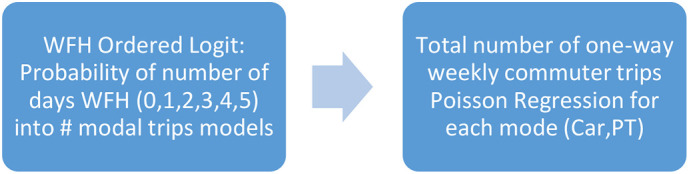
Two models are proposed (Fig. 10 ) as an appropriate contributing framework within which to study the behavioural linkages between WFH and commuting activity. The first model, an ordered choice logit model, represents the number of days each week an individual works from home. The second model, a Poisson regression for count data, defines the number of one-way weekly commuting trips by car and by public transport. The predicted probability of the number of days WFH is fed into the Poisson regression models for one-way weekly car and one-way weekly public transport commuting trips as a way of recognising its influence on the quantum of commuting activity. To correct the estimated asymptotic covariance matrix for the estimator at step 2 for the randomness of the estimator carried forward from the ordered logit WFH choice model, the standard Murphy and Topel (1985) correction is implemented, so that the standard errors of the Poisson model are asymptotically efficient.
Fig. 10.
The Model System.
For the ordered logit model, let Yi⁎ denote an unobserved (or latent) continuous variable (−∞ < Yi⁎ < +∞), defined in utility space, and μ0, μ1, …, μJ-1, μJ denote the threshold utility points in the distribution of Yi⁎, where μ0 = −∞ and μJ = +∞. Define Yi to be an ordinal (observed) variable for WFH such that Yi = j if μJ-1 ≤ Yi⁎ ≤ μJ;j = 1,2, …,J response levels. Since Yi⁎ is not observed, the mean and variance are unknown. Statistical assumptions must be introduced such that Yi⁎ has a mean of zero and a variance of one. To make the model operational, we define a relationship between Yi⁎ and Yi. The ordered choice model is based on a latent regression model given as eq. (1) (Winship and Mare, 1984; Greene and Hensher, 2010).
| (1) |
where θ collects the mean and threshold parameters. The observation mechanism results from a complete censoring of the latent dependent variable as follows:
| (2) |
The probabilities which enter the log likelihood function are given by eqs. (3) and (4).
| (3) |
| (4) |
The number of weekly one-way trips by car and public transport is a positive number compliant with a count model such as Poisson regression with latent heterogeneity. As a non-negative continuous count value, with truncation at zero, discrete random variable, Y, with observed trips, yn, (n observations), the Poisson regression model is given as eq. (5).
| (5) |
In this model, λn is both the mean and variance of yn; E[yn|xn] = λn. We allow for unobserved heterogeneity (see Greene, 2000). With a greatly reduced number of one-way weekly trips by car and public transport, there are many observations with zero commuting activity. We can allow for this using the ZIP form for count data (see Greene, 2000) to recognise the possibility of partial observability if data on weekly one-way trips being observed exhibits zero trips. In the current data under the pandemic, zero is in the main a legitimate value; however the ZIP form is still a valuable way of recognising this spike. We define z = 0 if the response would always be 0, 1 if a Poisson model applies; y = the response from the Poisson model; then zy = the observed response. The probabilities of the various outcomes in the ZIP model are:
| (6a) |
| (6b) |
The ZIP model is given as (Greene, 2017) Yn = 0 with probability qn and Yi ~ Poisson (λn) with probability 1 – qn so that.
| (7) |
| (8) |
where Rn(y) = the Poisson probability moel given in eq. (5). We assume that the ancillary, state probability, qn, is distributed normal; qn ~ Normal [vn]. Let F[vn] denote the normal CDF. Then,
| (9) |
Eq. (9) would, under ZIP, replace eq. (5) with a single new parameter which may be positive or negative. If there is no (or little) evidence of zero trips in any observations, then we do not expect the τ parameter to be statistically significant, and we can default to the Poisson form with normal latent heterogeneity.
6. Model results
6.1. The ordered logit model for the incidence of working from home
The final ordered logit models6 for WFH are summarised in Table 4, with an overview of the variables in the model provided in Table 3 . In selecting and testing candidate explanatory variables, we wanted to identify influences on WFH that relate to an employee's situation where they could choose to WFH or otherwise, with the position supported or enforced by their employer, under government restrictions in the early days of the COVID-19 lockdown as well as when restrictions began to be relaxed.
Table 4.
Ordered logit choice model for WFH.
| Wave 1 | Wave 2 | ||
|---|---|---|---|
| Units | Estimated parameter (t-value) | Estimated parameter (t-value) | |
| Constant | −0.6967 (−2.91) | −1.0330 (−7.94) | |
| Have a choice to work from home pre-COVID-19 | 1,0 | 2.1825 (7.83) | 0.5067 (4.65) |
| Employer directs employee to work from home post-COVID-19 | 1,0 | 2.9221 (11.30) | 1.5955 (14.5) |
| Type of work cannot be completed from home | 1,0 | −1.0764 (−3.66) | −0.7662 (−5.90) |
| Sydney/Melbourne/Brisbane metropolitan areas | 1,0 | 0.4519 (2.45) | |
| Urban location | 1,0 | – | 0.1448 (1.86) |
| Occupation (ABS 8 classes): | |||
| Technicians and trades | −0.8854(−1.75) | – | |
| Community and personal services | 1,0 | – | −0.5322 (−3.56) |
| Clerical and administration | 1,0 | – | −0.4874 (−5.15) |
| Sales | 1,0 | – | −0.4090 (−3.96) |
| Annual household income | $’000 s | 0.0026(1.97) | – |
| Attitudinal variables: | |||
| Productivity when WFH – lot less and little less | 1,0 | – | 0.4994 (4.78) |
| Productivity when WFH –little more and lot more | 1,0 | – | 0.8032 (7.76) |
| Appropriate space to work – strongly disagree, disagree & somewhat disagree | 1,0 | – | 1.9316 (12.9) |
| Appropriate space to work – somewhat agree, agree & strongly agree | 1,0 | – | 1.5685 (12.7) |
| WFH has a positive experience – strongly disagree, disagree & somewhat disagree | 1,0 | – | 1.1929 (7.85) |
| WFH has a positive experience - somewhat agree, agree & strongly agree | 1,0 | – | 0.6388 (4.67) |
| Like to WFH more often - strongly disagree, disagree & somewhat disagree | 1,0 | – | 0.8998 (4.97) |
| Like to WFH more often - somewhat agree, agree & strongly agree | 1,0 | – | 0.8912 (7.29) |
| I trust government to respond in the future – somewhat & strongly agree | 1,0 | – | −0.1554 (−1.83) |
| I will go to work from time to time – somewhat & strongly disagree | 1,0 | – | −0.4376 (−3.98) |
| I will go to work from time to time – somewhat & strongly agree | 1,0 | – | −0.5948 (−7.00) |
| Threshold parameters: | |||
| μ1 | 0.4924 (6.18) | 0.8688 (22.04) | |
| μ2 | 1.0620 (10.6) | 1.5639 (36.61) | |
| μ3 | 1.7127 (15.67) | 2.1140 (47.79) | |
| μ4 | 2.0349 (17.41) | 2.5414 (53.34) | |
| Goodness of Fit: | |||
| Pseudo-R2 | 0.221 | 0.314 | |
| Restricted log-likelihood | −766.05 | −6100.97 | |
| Log-likelihood at convergence | −596.34 | −4182.62 | |
| Sample Size | 476 | 705 |
Note: Mean probability of number of days per week WFH are W2 (W1): 0 days: 0.456 (0.381), 1 day: 0.018 (0.063), 2 days: 0.068 (0.075), 3 days: 0.058 (0.089), 4 days: 0.047 (0.046) and 5 days or more: 0.291(0.346).
Note: t-values are provided in brackets within each table and the 95% confidence intervals for each parameter estimate are available on request.
Table 3.
Descriptive Profile of WFH Model Variables, Waves 1 and 2.
| Variable (Mean (SD)) | Units | Wave 1 | Wave 2 |
|---|---|---|---|
| Number of days working from home | Number | 2.49 (2.20) | 2.18 (2.19) |
| Have a choice to work from home pre-COVID-19 | 1,0 | 0.181 | 0.203 |
| Employer directs employee to work from home post-COVID-19 | 1,0 | 0.347 | 0.306 |
| Type of work cannot be completed from home | 1,0 | 0.278 | 0.226 |
| Technicians and trades | 1,0 | 0.055 | 0.101 |
| Community and personal services | 1,0 | – | 0.180 |
| Clerical and administration | 1,0 | – | 0.162 |
| Sydney/Melbourne/Brisbane metropolitan areas | 1,0 | 0.455 | – |
| Urban location | 1,0 | – | 0.668 |
| Annual household income | $’000 s | 114 | – |
| Productivity when WFH – lot less and little less | 1,0 | – | 0.149 |
| Productivity when WFH –little more and lot more | 1,0 | – | 0.187 |
| Appropriate space to work – strongly disagree, disagree & somewhat disagree | 1,0 | – | 0.089 |
| Appropriate space to work – somewhat agree, agree & strongly agree | 1,0 | – | 0.404 |
| WFH has a positive experience – strongly disagree, disagree & somewhat disagree | 1,0 | – | 0.075 |
| WFH has a positive experience - somewhat agree, agree & strongly agree | 1,0 | – | 0.384 |
| Like to WFH more often - strongly disagree, disagree & somewhat disagree | 1,0 | – | 0.040 |
| Like to WFH more often - somewhat agree, agree & strongly agree | 1,0 | – | 0.377 |
| I trust government to respond in the future – agree & strongly agree | 1,0 | – | 0.757 |
| I will go to work from time to time – agree & strongly disagree | 1,0 | – | 0.174 |
| I will go to work from time to time – agree & strongly agree | 1,0 | – | 0.505 |
In developing behaviourally rich models to represent the extreme lockdown in the latter half of March (as captured in the Wave 1 data), and the late May Wave 2 context of partial relaxation of restrictions, we recognised that the key drivers of WFH and commuting activity between these two time periods are likely to be very different. Specifically, in late March the decision to WFH and cease commuting was largely driven by mandated government directives, but with the great majority of employees and employers supporting WFH unless it is was not a feasible option. Apart from employer policies which included employees having a choice to work from home pre-COVID-19, we anticipated that employee occupation and income may have a role in determining the extent of WFH. We also expected that in late March the shock to the system was still being digested by workers with very limited knowledge of whether WFH would work out, and what strategies governments were putting in place to minimise the risk of exposure to the virus.
As time moved forward between late March and late May, questions in the survey associated with an accumulated experience in WFH and gaining an understanding of the role that government played, started to take on real meaning as people crystallised their views now that they are better informed, and indeed are reflected in the statistical significance of a number of the attitudinal questions, in contrast to late March (Wave 1) where they had no behavioural relevance.
Both Wave 1 and Wave 2 models have overall goodness of fits within the range for pseudo-R2 typically obtained (i.e., 0.2 to 0.4) (Hensher et al., 2015). Both waves have identified three statistically significant employer-policy dummy variables, namely an employee having a choice to work from home pre-COVID-19, an employer directs the employee to work from home during COVID-19, and the type of work undertaken by the employee cannot be completed from home. The first two of the dummy variables have positive parameter estimates, suggesting that the probability of having more compared to less days of WFH increases when each of these policy settings are on offer; in contrast when the work cannot be completed at home, the probability of working away from home increases.
We considered all available socioeconomic characteristics (i.e., occupation, age, gender and household income), and found for Wave 1 that only one occupation class (i.e., technician and trades) based on the Australian Bureaus of Statistics 8-category Classification,7 and household income, were statistically significant indicators for establishing the extent to which WFH occurred. Technician and trade occupations tend to reduce the probability of WFH which makes good sense since such jobs typically include electricians, plumbers and builders. Household income has a positive parameter estimate, suggesting that as household income increases, we can expect a higher probability of being able to, and preferring to, WFH. The residential location of respondents was investigated, and we found that in Wave 1, people living in the three largest metropolitan areas in Australia (Sydney, Melbourne and Brisbane), tended to have a higher probability of WFH, which seems plausible given the mix of occupations compared to regional, rural and small city environments.
Wave 2 included 11 opinion and attitudinal variables together with three occupation classes that were not statistically significant in Wave 1. The three occupation classes (community and personal services, clerical and administration, and sales) were statistically significant while household income was not, suggesting that these occupation classes have a lower probability of working from home as restrictions start to relax and possibly as they are required to spend some amount of time back in the office.8 We also found that respondents residing in all capital cities had a higher probability of WFH.
The attitudinal variables are all coded as dummy variables relative to a ‘neutral’ opinion, as such the expectation on the sign is that it could be in either direction as these dummy variables now measure agreement or disagreement (rather than some level of agreement). For all attitudinal variables, it is important to emphasise that, in late May, we were still dealing with constrained choices in that people were being directed to work from home, and hence this effect as captured through the employer policy variables was having a significant and dominating influence on the extent of WFH (typically 40% of the sample were WFH 5 days a week) which in itself could prime views about working from home.
We find that productivity when WFH, associated with positive parameters, can be rationalised as follows: regardless of whether an individual believes that they are more or less productive when they WFH, they still prefer to do so, but the parameter estimate is significantly greater when productivity at home is perceived to be higher. The appropriateness of workspace at home also has positive parameters, suggesting that the less concern you have about your workspace, the more likely you are to work from home versus those that have a higher level of concern, but still a preference to WFH. On the positive experience associated with WFH, the positive parameter estimates follow a similar pattern; the more you work from home, probably the less (but still) positive you find it, given anecdotal evidence that a growing number of individuals are wanting some amount of social interaction in the workplace that is not possible online through videoconferencing and/or phone meetings. Indeed, the response to the desire to go to work from time to time, as negative parameters, reinforces the position of some likely increase in the probability of not working from home. Finally, the estimated parameter for trust in government responding to COVID-19 is negative, suggesting that as of late May, for those individuals who agreed with this statement, the greater the probability that they will be prepared to reduce the number of days working from home. This last point is powerful evidence of the importance of messaging by Government.
Although the parameter estimates are statistically significant, they are not behaviourally very interesting; instead care must be taken in interpreting the numerical magnitude of each parameter estimate since they are non-comparable in this non-linear logit form (Hensher et al., 2015). In Table 5 we present elasticities as a way of meaningfully comparing the influence of each explanatory variable on WFH. For the logit form, the elasticity of the probability is given in eq. (10) (Greene and Hensher, 2010).
| (10) |
Table 5.
Direct elasticity of choice.
| Working from Home Days per week: | 0 | 1 | 2 | 3 | 4 | 5 or more |
|---|---|---|---|---|---|---|
| Have a choice to work from home pre-COVID-19 | −0.301 (−0.817) | −0.056 (−0.726) | 0.136 (−0.546) | 0.281 (−0.145) | 0.372 (0.393) | 0.487 (2.715) |
| Employer directs employee to work from home post-COVID-19 | −0.875 (−1.213) | −0.244 (−0.720) | 0.269 (−0.405) | 0.745 (−0.097) | 1.119 (0.688) | 1.746 (3.233) |
| Type of work can be completed from home | 0.494 (0.605) | −0.044 (0.179) | −0.287 (−0.087) | −0.421 (−0.398) | −0.489 (−0.627) | −0.562 (−0.943) |
| Urban location | −0.091 (−0.269) | −0.004 (−0.146) | 0.049 (−0.024) | 0.082 (0.150) | 0.101 (0.297) | 0.122 (0.525) |
| Occupation (ABS 8 classes): | ||||||
| Technicians and trades | (0.541) | (0.087) | (−0.148) | (−0.387) | (−0.543) | (−0.724) |
| Community and personal services | 0.345 | −0.032 | −0.203 | −0.295 | −0.341 | −0.387 |
| Clerical and administration | 0.313 | −0.016 | −0.180 | −0.273 | −0.321 | −0.371 |
| Sales | 0.262 | −0.010 | −0.150 | −0.230 | −0.272 | −0.315 |
| Annual household income | (−0.188) | (−0.099) | (−0.013) | (0.109) | (0.210) | (0.358) |
| Productivity when WFH – lot less and little less | −0.295 | −0.061 | 0.129 | 0.276 | 0.369 | 0.488 |
| Productivity when WFH –little more and lot more | −0.459 | −0.122 | 0.177 | 0.426 | 0.597 | 0.832 |
| Appropriate space to work – strongly disagree, disagree & somewhat disagree | −0.857 | −0.527 | −0.078 | 0.521 | 1.155 | 2.769 |
| Appropriate space to work – somewhat agree, agree & strongly agree | −0.905 | −0.148 | 0.362 | 0.782 | 1.085 | 1.544 |
| WFH has a positive experience – strongly disagree, disagree & somewhat disagree | −0.612 | −0.281 | 0.110 | 0.526 | 0.871 | 1.468 |
| WFH has a positive experience - somewhat agree, agree & strongly agree | −0.388 | −0.048 | 0.189 | 0.356 | 0.458 | 0.581 |
| Like to WFH more often - strongly disagree, disagree &somewhat disagree | −0.483 | −0.192 | 0.128 | 0.439 | 0.676 | 1.042 |
| Like to WFH more often - somewhat agree, agree & strongly agree | −0.533 | −0.079 | 0.245 | 0.486 | 0.639 | 0.836 |
| I trust government to respond in the future – somewhat and strongly agree | 0.096 | 0.009 | −0.049 | −0.088 | −0.111 | −0.137 |
| I will go to work from time to time – disagree & strongly disagree | 0.281 | −0.012 | −0.161 | −0.246 | −0.290 | −0.336 |
| I will go to work from time to time – agree & strongly agree | 0.369 | 0.025 | −0.191 | −0.334 | −0.417 | −0.513 |
Note: Measures are associated with the number of days WFH with respect to given variable in Wave 2 (Wave 1 in brackets).
Note: The elasticity as a percent change equals the partial effect/probability of WFH for that response level. All elasticities are statistically significant at the 95% confidence level or better and are available on request.
where the marginal effect is given in eq. (11).
| (11) |
A marginal effect for continuous variables is the influence a one unit change in an explanatory variable has on the probability of selecting a particular outcome, ceteris paribus. For dummy (1,0) variables, which are the main variables in the models, the marginal effects are the derivatives of the probabilities given a change in the level of the dummy variable. The marginal effects need not have the same sign as the model parameters. Hence, the statistical significance of an estimated parameter does not imply the same significance for the marginal effect (see eq. 12). Neither the sign nor the magnitude of need bear any relationship to those of βj. βj, equal to ∂log(Pj/P0)/∂x, is commonly defined as an interpretation of the model parameters.
| (12) |
Looking first at the variables related to employer policy, the mean elasticity estimates suggest that the employer directive to WFH (associated with a government mandated restriction) has the greatest behavioural response, notably for WFH 4 and 5 days a week for both waves, and is noticeably much greater in Wave 1 (late March), as expected. There is evidence of the softening of the response in late May as we see restrictions relaxed, and possibly a greater appreciation of the risks of moving to some amount of not working from home.9 The negative elasticity estimated for WFH = 0 compared to the positive elasticity estimates for WFH 5 days a week is consistent with the view that having a choice to work from home or an employer directive to WFH, reduces the probability of going to work 5 days a week and increases the probability of WFH 5 days a week, with the latter a greater behavioural response.
A similar logic can be applied to all of the direct elasticity estimates. The household income elasticity estimates suggest that as household income increases, the probability of WFH 5 days under Wave 1 increases and decreases for WFH zero days per week. The elasticity estimates are generally greater and negative for the three employment policy variables in Wave 1 when there is WFH, and decline into the positive range for situations where there is commuting five or more days per week.
For the attitudinal variables associated with Wave 2 that have a positive parameter estimate in Table 4, we see that as we move from WFH 5 days a week to no days per week, that the behavioural responsiveness declines from a positive estimate for WFH equal to 2 to 5 days, to a negative estimate for 0 to 1 days. This is plausible and aligned with the interpretation of the Wave 2 model in Table 4 where the relaxation of restrictions is seeing a greater percentage change in the probability of WFH more days than less days over 2 to 5 days a week. The behavioural sensitivity associated with each explanatory variables is presented in more detail in a later section where we assess various scenarios.
In linking the WFH model to the modal trip frequency models, we have to calculate the probability of choosing a number of days WFH. The mean probability of each WFH level for Waves 2 and 1 (the latter in brackets) are 0 days: 0.456 (0.381), 1 day: 0.018 (0.063), 2 days: 0.068 (0.075), 3 days: 0.058 (0.089), 4 days: 0.047 (0.046), and 5 days or more: 0.29 (0.346). Given the estimated parameters obtained from the WFH ordered logit model, we can calculate the probabilities associated with each of the number of days working from home and enter them as explanatory variables into the Poisson regression model. These probabilities are obtained for each respondent using the following formulae, with an example given for four ordered alternatives.
Define Ufit = b(1) + b(2)*x1 + b(3)*x2 as the utility expression for a constant and two explanatory variables;
f0 = exp.(-Ufit)/(1 + exp.(-Ufit));
f1 = exp.(μ1- Ufit)/ (1 + exp.(μ1- Ufit));
f2 = exp.(μ2- Ufit)/(1 + exp.(μ2- Ufit));
p0 = f0; p1 = f1-f0; p2 = f2-f1; p3 = 1-f2; and.
pmodel = (y = 0)*p0 + (y = 1)*p1 + (y = 2)*p2 + (y = 3)*p3, where p = the choice probability for that level.
6.2. The Poisson regression model results for commuting activity
Turning to the Poisson regression model (in Table 7) with the number of weekly one-way modal trips defined as an integer for the Poisson count model, the overall goodness of fit (as pseudo R2) of all models are excellent for a non-linear model, varying from 0.369 to 0.681. A descriptive profile of the explanatory variables that are statistically significant is given in Table 6 . The sigma parameter that is estimated to allow for latent normal heterogeneity was statistically significant in all four models at the 1% level. Tau, the ZIP parameter is are statistically significant in Wave 2 but not in Wave 1. The Vuong statistics suggest that the estimated extended Poisson models in Table 7 for Wave 1 are favoured over an unaltered Poisson model. The Vuong statistics of 22.45 for car and 6.45 for public transport for Wave 2 also suggest that the estimated extended Poisson model is favoured over an unaltered Poisson model, but with censoring using Probit. That is, the dependent variable is over-dispersed and has an excessive number of zeros.10
Table 7.
Influence of WFH on number of weekly one-way modal commuter trips.
| Wave 1 | Wave 2 | |||
|---|---|---|---|---|
| Car | Public Transport | Car | Public Transport | |
| Constant | 0.468 (3.64) | −2.114 (−9.1) | 0.7060 (6.27) | −0.2421 (−5.39) |
| Annual household income ($000 s) | 0.0035 (4.49) | −0.0207 (−15.6) | 0.0032 (12.95) | −0.0036 (−4.59) |
| Professionals (ABS 8 classes) | 0.498 (5.37) | 0.1675 (4.74) | 0.3321 (4.03) | |
| Metro Location (Sydney, Brisbane, Melbourne) (1,0) | – | – | – | 1.4878 (5.86) |
| Other capital cities (1,0) | – | – | – | 0.4782 (3.80) |
| Urban (including metro and capital cities) (1,0) | – | – | 0.0690 (1.99) | – |
| Male (1,0) | – | 1.231 (12.23) | – | – |
| Health risk to me personally (10 = extremely high) | – | – | −0.0014 (−1.61) | – |
| Probability WFH 0 days per week | 1.094 (5.97) | −1.9408 (−9.96) | 1.4043 (24.29) | 0.4303 (3.53) |
| Probability WFH 1 day per week | – | – | 1.6014 (4.40) | – |
| Tau (ZIP) | – | – | −0.3265 (−25.20) | −0.8627 (−2.93) |
| Sigma (latent heterogeneity) | 1.322 (19.9) | 3.5322 (18.96) | 0.7274 (38.62) | 1.9176 (27.40) |
| Goodness of fit | ||||
| Pseudo R2 | 0.404 | 0.671 | 0.369 | 0.681 |
| Vuong stat vs Poisson | 9.33 | 4.605 | 24.25 | 6.485 |
| Partial effects | ||||
| Annual household income ($000 s) | 0.031 (4.28) | −0.378 (−6.1) | 0.008 (12.9) | −0.0004 (−6.31) |
| Professionals (ABS 8 classes) | – | 9.12 (4.54) | 0.408 (4.72) | 0.0394 (4.12) |
| Urban (including metro and capital cities) (1,0) | – | – | 0.1680 (1.98) | |
| Metro Location (Sydney, Brisbane, Melbourne) (1,0) | – | – | – | 0.177 (8.44) |
| Other capital cities (1,0) | – | – | – | 0.0568(5.03) |
| Male (1,0) | – | 22.54 (7.41) | – | – |
| Health risk to me personally (10 = extremely high) | – | – | −0.003 (−2.2) | – |
| Probability WFH 0 days per week | 9.81 (5.22) | −35.53 (−5.24) | 3.418 (23.1) | 0.0511 (4.92) |
| Probability WFH 1 day per week | – | – | 3.897(4.41) | – |
Note: Vuong test favours extended model; Murphy and Topel correction of standard errors. The constants in the models were calibrated to match the predicted average trips to the actual average trips in the sample.
Note: t-values are provided in brackets within each table and the 95% confidence intervals for each parameter estimate are available on request.
Table 6.
Descriptive profile of commuter trips model variables.
| Wave 1 | Wave 2 | |||
|---|---|---|---|---|
| Car | Public Transport | Car | Public Transport | |
| One-way weekly commuting trips | 1.25 (3.03) | 0.60 (2.18) | 4.54 (5.78) | 0.887 (5.57) |
| Annual household income ($000 s) | 114 | 104 | ||
| Professionals (ABS 8 classes) (1,0) | 0.400 | 0.372 | ||
| Metro Location (Syd, Brs, Mel) (1,0) | – | 0.424 | ||
| Other capital cities (1,0) | – | 0.244 | ||
| Male (1,0) | 0.532 | – | ||
| Health risk to me personally (10 = extremely high) | – | 8.25 (1.78) | ||
| Probability WFH 0 days per week | 0.381 | 0.456 | ||
| Probability WFH 1 day per week | – | 0.082 | ||
Annual household income was found to be statistically significant for car and public transport trips in both Wave 1 and Wave 2. The positive sign for the car models is indicative of a greater number of weekly one-way trips for higher income households; in contrast the negative sign in the public transport models suggests fewer public transport trips for higher income households. The only other socioeconomic influences that were statistically significant are associated with the professional occupation (relative to all other occupations)11 and males for Wave 1 public transport, both positive; and professionals for Wave 2 use of both car and public transport, being also positive for both car and public transport.
Residential location was statistically significant in Wave 2, with all urban locations being statistically significant at the same level for car, but a separation of the main metropolitan locations from other capital cities for public transport produced only a marginal difference. The positive parameter estimate in the car model suggests more trips per week in all urban locations compared to regional and rural contexts. This result, may in part be attributable to generally more activity in urban areas but also because of less replacement of car travel with active transport modes. For public transport, the statistical significance was found to exist for separate variables for the three largest capital cities and other capital cities. The difference seems plausible given the greater availability of public transport in the larger cities, but also relatively good public transport in other capital cities compared to rural and regional locations. The public transport distinction compared to car, with a single parameter estimate for urban locations, is suggestive of the lack of influence of public transport on many car user preferences.
The probability of working from home no days a week was statistically significant in both waves for those using car and public transport. In both waves, it was positive for car use suggesting that as expected, all other influences remaining unchanged, as the probability of going to work 5 days a week increases, the number of one-way car commuter trips increases. For car in Wave 2, we also see a higher probability of going to work 4 days a week adding to the total switch back to the workplace. Under COVID-19 with biosecurity a concern, this makes good sense. However, for public transport, we observe a negative sign in Wave 1 which makes sense given that this was at the height of restrictions with government advice to not use public transport; but this changed to a positive sign in Wave 2 when a return, to some extent, to work resulted in an increase in public transport commuting trips, with social distancing in public transport requiring sitting only on seats with an allowable sitting sign.12 We might anticipate a continuing increase in public transport in ensuing periods as additional capacity is released and the growing evidence of PT being a relatively safe environment increases together with more positive government policy messaging. Finally, for wave 2 only, we obtained a negative sign associated with car use for the question on whether an individual sees a health risk personally to themselves under COVID-19. Although only marginally only statistically significant, this supports the position of an individual whose ranking of health risk is high, so undertaking fewer one-way commuter trips per week for car, translated into reduced commuting.
Given that the dependent variable is a count variable, and Poisson regression models the log of the expected number of weekly trips as a function of the predictor variables, we can interpret an estimated parameter as follows (Wooldridge, 2002): for a one unit change in the predictor variable, the difference in the logs of expected counts is expected to change by the respective parameter, given the other predictor variables in the model are held constant. For a binary variable such as gender, the difference in the logs of the expected number of weekly public transport trips in late March (Wave 1) is expected to be 1.231 higher for males compared to females, ceteris paribus. For a continuous explanatory variable such as the probability of WFH one day a week in late May (Wave 2), if a commuter were to increase the probability of WFH 1 day a week from say 0.1 to 0.2, the difference in the logs of expected number of weekly car trips would be expected to increase by 1.404 trips, ceteris paribus.
A more informed way of illustrating the behavioural response for one way weekly commuting trips associated with changes in the probability of WFH and other influences is to undertake a number of scenario applications, which we now present and discuss in the following section.
7. Simulating working from home and expected commuting trips
Using the models for Wave 1 and Wave 2, we simulate and test selected scenarios to examine the impact of any possible changes in predictors to the outcomes of WFH and commuting trips. We have selected several scenarios to illustrate the application of the models. We first examine the potential impact when different proportions of the workforce were directed to work from home (Scenario One). We also examined different levels of agreement on WFH related statements and the implications they are predicted to have on the average number of days WFH (Scenario Two). In predicting the numbers of trips by car, we applied a range of probabilities of WFH for 0 days to observe the related influence on the one-way weekly commuting trips by car (Scenario Three), and commuting trips by public transport (Scenario Four).
7.1. Scenario one: the impact of workforce directed to WFH
In this and the following four sections, we have focussed only on Wave 2 primarily because we want to speculate, through simulation, what the next period, under increasingly relaxed restrictions, might look like, and that the best data we have to make such predictions is Wave 2. The further justification is that Wave 1 is a very unusual case of immensely suppressed travel regardless of situation, attitude, work, etc. It is a baseline of “nothing” with few freedoms to vary anything. The simulation using Wave 2 produces more differentiated results compared to Wave 1, given the enhanced variability in the data.
Let us assume that all work can be performed from home instead of the sample average of 78% for Wave 2, which means all work theoretically can be completed by WFH if people were directed to do so. We simulated a scenario wherein 20% and up to 80% of the workforce were directed to work from home, to imitate the different phases of the lockdown or social distancing requirements at the workplace. In this scenario, the average number of WFH days would increase from 2.04 for 20% to 4.02 for 80%, a noticeable increase. The results are shown in Fig. 11 .
Fig. 11.

Impact of proportions of people directed to WFH on average number of days of WFH.
7.2. Scenario two: the impact of attitudes and experience on WFH
Using the evidence on individual's attitudes towards various aspects of the COVID-19 lockdown, and coming out of the initial height of the pandemic in late May as some restrictions are relaxed, we simulated changes in the response to the relevant scale used to measure attitudes: relative productivity; appropriateness of home working space; how positive WFH has been experienced, willingness to WFH more in the future. We varied the level of agreement for these statements from 20% to 80% to assess the impact on the average days WFH, as shown in Fig. 12 .
Fig. 12.

Impact of agreement levels on average days WFH.
We see that the most influential perspective regarding WFH choice is having adequate work space at home. The more a respondent agrees to this statement, the more likely they are willing to spend more days WFH. Conversely, low levels of agreement result in the lowest uptake of WFH days (1.6 days compared to all other statements if there was only 20% of agreement). Having a positive experience with WFH on the other hand, has a relatively small role in increasing the average WFH days compared to having adequate space and being productive. This may be a result of the fact that for many, WFH is currently a necessity rather than a choice, hence personal preference and experience play a relatively more minor role. Alternatively, it might also be the case that very few people disagreed with the statement (15%), and such limited ill-will towards the experience has meant that there is insufficient variability in negative experience to estimate a sizeable impact resulting from a bad experience at this stage. If individuals expressed a desire to want to go to work from time to time to avoid social isolation, the average number of WFH days would decline from 2.3 days at the 20% agreement level to 1.8 days at the 80% agreement level.
7.3. Scenario three: the impact of WFH on the number of one-way commuting car trips
Using the estimated ordered logit model, we predicted the probabilities that people would work from home zero days per week and what this might mean for the number of predicted weekly one-way car commuting trips. We assume that the average number of WFH days would vary and that its composition may also change over time with the tightening or easing of restrictions. We simulated a scenario with 20% to 80% of people not working from home at all (i.e., WFH 0 days).There is a noticeable increase of one-way weekly commuting trips from 3 trips to 7.8 trips when the proportion of workforce not working from home increases from 20% to 80%, as shown in Fig. 13 .
Fig. 13.

The increase in car commuting trips with a decrease in WFH.
The responsiveness of car travel in Wave 2 is likely to be a function of the easing of restrictions that occurred between Wave 1 and Wave 2, giving respondents more flexibility to vary their travel behaviour, within the parameters of the restrictions. Another explanation for the faster uptake in car travel for commuting is that in Wave 2, as more people start to travel, the private car becomes a preferred alternative during a pandemic for reasons of hygiene and the concern thereof related to public transport. For some individuals who used to take public transport pre-COVID-19, the choice would shift to commuting by car for this period, with an ongoing concern as to whether they will return to public transport at a later date.
7.4. Scenario four: the impact of WFH on the number of on-way commuting public transport trips
For Wave 2, the ZIP models for PT trips predicted a low level of commuting trips by public transport, at 0.89 predicted trips on average. Commuting by public transport during a pandemic lockdown period is not a preferred (or indeed desirable) choice, aided by government messaging to stay away from using public transport. A similar scenario as in Section 5.3 for car, was investigated for PT trips. The increase of PT trips is much slower than the increase for car trips when the proportion of the workforce not working from home increases from 20% to 80% (Fig. 14 ). This shows at least based on the answers taken during Wave 2 that people had no confidence to take more PT trips even if the restrictions were eased and more people were required to not work from home.
Fig. 14.

The increase in public transport commuting trips with a decrease in WFH.
This shows that regardless of where people are and whether they work more or less from home, the commuting choice using public transport is not generally preferred for now (up to late May), despite the slow return.
7.5. Different occupations and WFH and commuting trips
We identified the influence of specific occupation categories on the probability of working for home and also on the number of one-way weekly trips by car and public transport. During Wave 2 when, on average, 2.19 days people worked from home, in the ordered logit model we found that three occupation groups went back to the workplace more often than others, and hence worked less from home. They are community and personal services workers (WFH 1.80 days), clerical and administration staff (WFH 1.86 days), and sales workers (WFH 1.97 days). Many of their duties require interacting with others and hence are more difficult to do away from the work off-site.
Occupation not only directly affects WFH choices, it also directly influences the quantum of one-way weekly commuting trips. In the Wave 2 model, for car trips, professionals were predicted to have a higher level of one-way weekly commuting trips at 5.13 trips (approximately two one-way trips for two days) compared to 4.54 trips on average. They also commute more by public transport, with predicted 1.19 PT trips compared to 0.89 PT trips on average for the overall sample.
8. Discussion and future research
As we move away from the COVID-19 spike and the constrained travel observed in Wave 1, we see the signs of a movement in behaviour in Wave 2 which was collected after a month of a relatively low number of new cases of COVID-19 in Australia. While the general volume of work remains largely unchanged between the waves (with less work available as measured in the number of days worked in a week), we do see a slow move away from levels of work from home observed in Wave 1 towards those that existed prior to the outbreak of COVID-19. Overall however, the experience with working from home has been largely positive with the majority of respondents finding they have the space to do so, that they are generally as productive at home as they would be at work, and crucially there is an attitude that most respondents would like to work from home more in the future and even more so, a positive attitude towards the desire to commute at times when it not as busy. As a result, looking forward, there is an intention from respondents to work at home, on average, more days in the future than they did prior to COVID-19 along with a shift in the time of day of some car trips.
While behaviours are still relatively constrained, we do observe that in Wave 2 there is more variability in the data and hence an increasing number of variables that can explain the differences in working from home and the commuting trips undertaken. The ongoing monitoring of commuting will be crucially important; while we can already see an intention to start to travel to work more often than is currently the case, but less often than pre-COVID-19 levels, the level of variability in this planned behaviour is very large (our guess is that as restrictions are eased behaviours will remain quite variable for some time).
We also start to see the attitudes of the individual playing a role in determining the levels of working from home. A positive experience with working from home, and the desire to do so more often, all increase the probability of working from home more often. Most important is the availability of an appropriate space to work from home. Any support that can be given to make the home more conducive to work in the short-term will improve the experience, productivity and thus incidence of work from home, and will likely make it a longer term lever in the congestion management tool kit. Given that trust in government response is significant, any support given in this regard will likely strengthen this attitude too. We see a desire to maintain some level of work from home that is greater than it was previously, and as restrictions ease and the work from home experience crystallises, we may find that preferences of the individual start to drive variations in behaviour more significantly.
With regards to future research that will address some of the limitations of this study, ongoing analysis is needed as behaviours are still in a great state of change. The work from home experience for many is new and forced upon them, and most are still likely trying to come to grips with the change while balancing changes on a range of other fronts like the education of their children, the work status of their partner, and so on. We acknowledge that in these early stages, there is a high probability of cognitive dissonance, and we may see that the constrained “choice” to work from home may be determining current attitudes rather than attitude determining behaviour. This is clearly an area that requires more research by the wider community. Nonetheless, it is reasonable that having an appropriate space to work at home will be a key determinant in the choice to do so. To that end, more research is also needed to understand what defines an appropriate space and if it is possible that that space can be created. More work is also needed on the future of commuting via public transport. At present, that behaviour still remains significantly depressed, and more insight is need as to how public transport may begin to attract users again.
Overall, this paper presents an approach to modelling the impact of work from home within a framework that provides plausible and importantly, usable results in the context of travel demand forecasting. While the sample size is relatively small in the context of more formal travel demand models for strategic transport decisions, the sample of 476 respondents taken from Wave 1 and 705 from Wave 2 are sizeable enough to provide a robust proof of concept for utilisation on larger samples or wider studies of travel behaviour.
9. Conclusion
Overall, this paper provides the first insights into what will be an ongoing project to look at the impact of COVID-19 on working from home and commuting. Our modelling indicates that working from home will be a key determinant on commuting behaviour, and as restrictions are relaxed, we can expect to see a quicker increase in commuting trips by car, ceteris paribus. Therefore, understanding the determinants of work from home will be vital as we move forward. In modelling the number of days worked from home we find, unsurprisingly, that the role of the employer is of great importance. The ability to choose to work from home, or the direction to do so, is a large determinant of the number of days worked. If transport authorities wish to keep commuting trips at the current low levels, particularly given the modelled resistance to public transport that currently exists, then governments should encourage ongoing employer support (linked to sustainability goals) for working from home and for those organisations who are currently not allowing staff to do so, they should work with them to identify the barriers and help develop strategies to overcome them if indeed those barriers can be removed. It is interesting to note that working from home is generally more possible for those in urban areas and households with higher incomes, likely because of the nature of employment among these groups of individuals. Perhaps understanding potential barriers that can be overcome is more urgent for those outside these groups.
Acknowledgments
Acknowledgments
We thank the University of Sydney Business School for its financial support in funding the collection of Wave 2 data. This research is part of an ongoing iMove Cooperative Research Centre (CRC) research project 1-031 with Transport and Main Roads, Queensland, on Working for Home (WFH) and Implications for Revision of Metropolitan Strategic Transport Models. We also thank Kevin O'Connor and a referee for very useful suggestions to improve the paper.
Author contributions
Matthew Beck: Conceptualization; Data curation; Formal analysis; Funding acquisition; Investigation; Methodology;
Visualization; Roles/Writing - original draft; Writing - review & editing.
David Hensher: Conceptualization; Formal analysis; Funding acquisition; Investigation; Methodology; Project administration; Roles/Writing - original draft; Writing - review & editing.
Edward Wei: Formal analysis; Software; Supervision; Roles/Writing - original draft.
Footnotes
Which has been increased by an additional 10 days in NSW, Victoria and Queensland if after Day 11 these individuals refuse to undertake a swab test, with up to 20% of such persons refusing in Melbourne, the new hotspot.
On July 6, the NSW government announced that the closing of the borders with Victoria until the number of cases associated with this new ‘bump or spike’ of over 100 cases per day are under control.
The number of monthly trips by train and bus in NSW in April slumped to just 18% of peak use during 2020 (from 66.1 million trips to 11.6 million), in May that number had rebounded somewhat to 27% of peak use, rising to 17.8 million trips (https://www.transport.nsw.gov.au/data-and-research/passenger-travel/public-transport-patronage) These figures refer to all trip purposes and we expect that commuting activity decreased even more.
Approximately 68% of the sample reside in capital cities and the balance in rural/regional locations.
We estimated a commuter mode choice model for Wave 2 but decided not to include it at this stage since we believe it requires more time for travel behaviour to further adjust; we plan to revisit this model (and some extensions to the WFH model to recognise specific days of WFH and the staggered nature of commuting times) with the collection of Wave 3 data in late July.
We investigated various models with random parameters, and only three variables were statistically significant (namely employer directs employee to work from home post-COVID-19, productivity when WFH – lot less and little less, and productivity when WFH –little more and lot more), resulting in a slightly lower log likelihood at convergence of −4180.9 compared to Table 4 of −4182.62, with 3 degrees of freedom difference; and they had almost no influence on the simulated findings in Section 5. We will continue to explore different model types as data becomes richer and behaviours more varied.
Anecdotally, we note that many of these positions are relatively junior or are middle management, with senior management requiring some amount of return to the office or out in the field.
This will be an important behavioural feature to track as we add extra waves of data over the next 8 months.
We might have expected this same effect in Wave 1, given so little trip activity, but we were not able to identify a statistically significant estimate for tau.
Although a number of other occupations are already accounted for through the probability of working from home estimates.
In late May, this amounted to a 2% level of capacity compared to pre-Covid-19.
References
- ABS Labour Force, Australia, Australian Bureau of Statistics (Cat. No. 6333.0), August 2019. 2020. https://www.abs.gov.au/AUSSTATS/abs@.nsf/DetailsPage/6333.0August%202019?OpenDocument accessed 30/07/20.
- ABS . 2020. Persons Employed at Home, Australian Bureau of Statistics (Cat. No. 6275.0), July 2020.https://www.abs.gov.au/ausstats/abs@.nsf/c453a8b3c06b8023ca257090001f5c1d/ba7ce1e7d938a270ca256bd0002741d7!OpenDocument accessed 30/07/20. [Google Scholar]
- ABS . 2020. Employment, hours worked and unemployment rose in June 16/07/20.https://www.abs.gov.au/ausstats/abs@.nsf/lookup/6202.0Media%20Release1Jun%202020#:~:text=6202.0%20%2D%20Labour%20Force%2C%20Australia%2C%20Jun%202020&text=Seasonally%20adjusted%20employment%20increased%20by Bureau%20of%20Statistics%20(ABS), accessed 13/08/20. [Google Scholar]
- Anders G. Linkedin Workforce Insights; 2020. Workforce Confidence Index: Introducing a Biweekly Pulse on the Mood of Workers.https://www.linkedin.com/pulse/workforce-confidence-index-introducing-biweekly-pulse-george-anders (accessed 13/08/20) [Google Scholar]
- Beck M., Hensher D.A. Transport Policy; 2020. Insights into the Impact of COVID-19 on Household Travel and Activities in Australia – The Early Days of Easing Restrictions. (online August) [DOI] [PMC free article] [PubMed] [Google Scholar]
- Beck M.J., Hensher D.A. Insights into the impact of COVID-19 on household travel, work, activities and shopping in Australia – the early days under restrictions. Transp. Policy. 2020;96:76–93. doi: 10.1016/j.tranpol.2020.07.001. [DOI] [PMC free article] [PubMed] [Google Scholar]
- Ben-Akiva M., Bowman J.L., Gopinath D. Travel demand model system for the information era. Transportation. 1996;23:241–266. [Google Scholar]
- Brewer A., Hensher D.A. Distributed work and travel behaviour: the dynamics of interactive agency choices between employers and employees. Transportation. 2000;27(1):117–148. [Google Scholar]
- van den Broek D., Keating E. Rights to a process for the masses or select privileges for the few? Telework policy and labour market inequality in Australia. Policy Studies. 2009;32(1):21–33. [Google Scholar]
- Craig L., Churchill B. Dual-earner parent couples’ work and care during COVID-19. Gender, Work and Organisation, forthcoming. 2020 doi: 10.1111/gwao.12497. [DOI] [PMC free article] [PubMed] [Google Scholar]
- Derwin J. The Australian unemployment rate shot up to 7.1% in May as another 227,000 jobs were wiped out, 18/06/20. 2020. https://www.businessinsider.com.au/australian-unemployment-rate-job-losses-may-covid19-2020-6
- Dockery A.M., Bawa S. When two worlds collude: working from home and family functioning in Australia. International Labour Review. 2018;157(4):609–630. [Google Scholar]
- DSS Household, Income and Labour Dynamics in Australia. 2020. https://www.dss.gov.au/national-centre-for-longitudinal-data/household-income-and-labour-dynamics-in-australia-hilda-fact-sheet
- Greene W.H. Prentice Hall; Englewood Cliffs: 2000. Econometric Analysis. [Google Scholar]
- Greene W.H. Econometric Software Inc.; New York and Sydney: 2017. Limdep Version 10, Econometric Modelling Guide. [Google Scholar]
- Greene W.H., Hensher D.A. Cambridge University Press; Cambridge, April: 2010. Modeling Ordered Choices: A Primer and Recent Developments. [Google Scholar]
- Hall D.T. Paper Prepared for the Annual Review of Communications and Society, a Joint Project of the Aspen Institute and the Institute for Information Studies. Boston University; August: 1989. Telecommuting and the management of work-home boundaries. [Google Scholar]
- Hensher D.A., Golob J. Elsevier Science; Oxford: 2002. Telecommunications-Travel Interaction: Workshop Report in Mahmassani, H. (Ed.) In Perpetual Motion: Travel Behavior Research Opportunities and Application Challenges; pp. 209–219. [Google Scholar]
- Hensher D.A., Rose J.M., Greene W.H. Second edition. Cambridge University Press; Cambridge: 2015. Applied Choice Analysis. [Google Scholar]
- Hopkins J.L., McKay J. Investigating ‘anywhere working’ as a mechanism for alleviating traffic congestion in smart cities. Technol. Forecast. Soc. Chang. 2019;142:258–272. [Google Scholar]
- Kim S.N., Choo S., Mokhtarian P.L. Home-based telecommuting and intra-household interactions in work and non-work travel: a seemingly unrelated censored regression approach. Transp. Res. A. 2015;80:197–214. [Google Scholar]
- Lister K. Latest Work-at-Home/Telecommuting/Mobile Work/Remote Work. 2020. https://globalworkplaceanalytics.com/telecommuting-statistics
- Mokhtarian P.L. Telecommuting and travel: state of the practice, state of the art. Transportation. 1991;18:319–342. [Google Scholar]
- Mokhtarian P.L., Handy S.L., Salomon I. Methodological issues in the estimation of the travel, energy and air quality impacts of telecommuting. Transp. Res. A. 1995;29(4):283–302. [Google Scholar]
- Mokhtarian P.L., Collantes G.O., Gertz C. Telecommuting, residential location, and commute-distance traveled: evidence from state of California employees. Environ Plan A. 2004;36(10):1877–1897. [Google Scholar]
- Murphy K., Topel R. Estimation and inference in two-step econometric models. J. Bus. Econ. Stat. 1985;3(4):370–379. [Google Scholar]
- Nash M., Churchill B. Caring during COVID-19: a gendered analysis of Australian university responses to managing remote working and caring responsibilities. Gender, Work and Organisation, forthcoming. 2020 doi: 10.1111/gwao.12484. [DOI] [PMC free article] [PubMed] [Google Scholar]
- Nilles J.M. John Wiley & Sons; New York, United States: 1973. Telecommunications-Transportation Tradeoff: Options for Tomorrow. [Google Scholar]
- Paleti R., Vukovic I. Telecommuting and its impact on activity-time use patterns of dual-earner households. Transp. Res. Rec. 2017;2658:17–25. [Google Scholar]
- Paul K. 2020. Twitter announces employees will be allowed to work from home ‘forever’.https://www.theguardian.com/technology/2020/may/12/twitter-coronavirus-COVID19-work-from-home The Guardian 13/05/2020. (accessed 27/05/20) [Google Scholar]
- Roy Morgan . 2020. Over two-thirds of working Australians have had their employment impacted by the ‘Coronavirus Crisis’ 24/04/20.http://www.roymorgan.com/findings/8383-roy-morgan-coronavirus-crisis-impact-on-employment-april-24-2020-202004240654 accessed 13/08/20. [Google Scholar]
- Salomon I. Telecommunications and travel relationships: a review. Transp. Res. 1986:223–238. 20A. [Google Scholar]
- Salomon I, Salomon M. Telecommuting: The employee’s perspective. Technological Forecasting and Social Change. 1984;25(1):15–28. [Google Scholar]
- Sener I.N., Bhat C.R. A copula-based sample selection model of telecommuting choice and frequency. Environ Plan A. 2011;43:126–145. [Google Scholar]
- Singh P., Paleti R., Jenkins S., Bhat C.R. On modeling telecommuting behavior: Option, choice, and frequency. Transportation. 2013;40:373–396. [Google Scholar]
- Smith, P. (2020) Westpac mulls permanent remote staff. Financial Review 12/05/20, https://www.afr.com/technology/westpac-mulls-permanent-remote-staff-20200507-p54qri, (accessed 27/05/20).
- Treasury . Australian Government Treasury; 2020. Economic Response to the Coronavirus - JobKeeper Postcode Data.https://treasury.gov.au/coronavirus/jobkeeper/data (accessed 13/08/20) [Google Scholar]
- Troup C., Rose J. Working from home: do formal or informal telework arrangements provide better work–family outcomes? Community Work Fam. 2012;15(4):471–486. [Google Scholar]
- Wilton R.D., Páez A., Scott D.M. Why do you care what other people think? A qualitative investigation of social influence and telecommuting. Transp. Res. A. 2011;45:269–282. [Google Scholar]
- Winship C., Mare R. Regression models with ordinal variables. Am. Sociol. Rev. 1984;49:512–525. [Google Scholar]
- Wooldridge J.M. MIT Press; Cambridge: 2002. Econometric Analysis of Cross Section and Panel Data. [Google Scholar]
- Yen J.R., Mahmassani H. Telecommuting adoption: conceptual framework and model estimation. Transp. Res. Rec. 1997;1606:95–102. [Google Scholar]
- Zhu P. Are telecommuting and personal travel complements or substitutes? Ann. Reg. Sci. 2012;48:619–639. [Google Scholar]