Photo Credit: Cathy Händel, Published on http://www.suttonelms.org.uk/olla12.html
Sometimes when you’re looking for something else, you happen across an even more exciting result. That’s what’s happened at LHCb, illustrated in the paper “Observation of \(J/\psi p\) resonances consistent with pentaquark states in \(\Lambda_b^0\to J/\psi K^-p\) decays”, released on the arXiv on the 14th of July.
I say this is lucky because the analysts found these states while they were busy looking at another channel; they were measuring the branching fraction of \(B^0\to J/\psi K^+ K^-\). As one of the analysts, Sheldon Stone, recalled to me, during the review of the \(B^0\) analysis, one reviewer asked if there could be a background from the decay \(\Lambda_b^0\to J/\psi K^- p\), where the proton was misidentified as a kaon. As this was a viable option, they looked at the PDG to see if the mode had been measured, and found that it had not. Without a certain knowledge of how large this contribution would be, the analysts looked. To their surprise, they found a rather large rate of the decay, allowing for a measurement of the lifetime of the \(\Lambda_b^0\). At the same time, they noticed a peak in the \(J/\psi p\) spectrum. After completing the above mentioned analysis of the \(B^0\), they returned to the channel.
It’s nice to put yourself in the analysts shoes and see the result for yourself. Let’s start by looking at the decay \(\Lambda_b^0\to J/\psi p K^-\). As this is a three body decay, we can look at the Dalitz Plots.
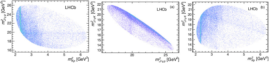
Dalitz plots from the decay \(\Lambda_b^0\to J/\psi K^- p\). Compiled from http://arxiv.org/abs/1507.03414
The above Dalitz plots show all combinations of possible axes to test. In the one on the left, around \(m^2=2.3\) GeV\(^2\), running vertically, we see the \(\Lambda(1520)\) resonance, which decays into a proton and a kaon. Running horizontally is a band which does not seem to correspond to a known resonance, but which would decay into a \(J/\psi\) and a proton. If this is a strong decay, then the only option is to have a hadron whose minimum quark content is \(uud\bar{c}c\). The same band is seen on the middle plot as a vertical band, and on the far right as the sloping diagonal band. To know for sure, one must perform a complete amplitude analysis of the system.
You might be saying to yourself “Who ordered that?” and think that something with five quarks hadn’t been postulated. This is not the case. Hadrons with quark content beyond the minimum were already thought about by Gell-Mann and Zweig in 1964 and quantitatively modeled by Jaffe in 1977 to 4 quarks and 5 quarks by Strottman in 1979. I urge you to go look at the articles if you haven’t before.
It appears as though a resonance has been found, and in order to be sure, a full amplitude analysis of the decay was performed. The distribution is first modeled without any such state, shown in the figures below.

Projections of the fits of the\( \Lambda_b^0\to J/\psi K^- p\) spectrum without any additional components. Black is the data, and red is the fit. From http://arxiv.org/abs/1507.03414
Try as you might, the models are unable to explain the invariant mass distribution of the \(J/\psi p\). Without going into too much jargon, they wrote down from a theoretical standpoint what type of effect a five quark particle would have on the Dalitz plot, then put this into their model. As it turns out, they were unable to successfully model the distribution without the addition of two such pentaquark states. By adding these states, the fits look much better, as shown below.

Mass projection onto the \(J/\psi p\) axis of the total fit to the Dalitz plot. Again, Black is data, red is the fit. The inset image is for the kinematic range \(m(K p)>2 GeV\).
From http://arxiv.org/abs/1507.03414
The states are called the \(P_c\) states. Now, as this is a full amplitude analysis, the fit also covers all angular information. This allows for determination of the total angular momentum and parity of the states. These are defined by the quantity \(J^P\), with \(J\) being the total angular momentum and \(P\) being the parity. All values for both resonances are tried from 1/2 to 7/2, and the best fit values are found to be with one resonance having \(J=3/2\) and the other with \(J=5/2\), with each having the opposite parity as the other. No concrete distinction can be made between which state has which value.
Finally, the significance of the signal is described by under the assumption \(J^P=3/2^-,5/2^+\) for the lower and higher mass states; the significances are 9 and 12 standard deviations, respectively.
The masses and widths turn out to be
\(m(P_c^+(4380))=4380\pm 8\pm 29 MeV\)
\(m(P_c^+(4450))=4449.8\pm 1.7\pm 2.5 MeV\)
With corresponding widths
Width\((P_c^+(4380))=205\pm 18\pm 86 MeV\)
Width\((P_c^+(4450))=39\pm 5\pm 19 MeV\)
Finally, we’ll look at the Argand Diagrams for the two resonances.

Argand diagrams for the two \(P_c\) states.
From http://arxiv.org/abs/1507.03414
Now you may be saying “hold your horses, that Argand diagram on the right doesn’t look so great”, and you’re right. I’m not going to defend the plot, but only point out that the phase motion is in the correct direction, indicated by the arrows.
As pointed out on the LHCb public page, one of the next steps will be to try to understand whether the states shown are tightly bound 5 quark objects or rather loosely bound meson baryon molecule. Even before that, though, we’ll see if any of the other experiments have something to say about these states.